Chunking Analysis: Which is the right chunking approach for your language?

Before we get into specific chunking approaches, we should first ask whether chunking depends on the language at all and how much chunking affects retrieval across languages when building RAG applications.

Many teams use the same chunking approach for every language, and often it works—but is it actually right? Do we have evidence to back that choice? In this post, we’ll explore that by answering two questions:

1. Does chunking depend on the language?
2. Which is the right chunking approach for your language?

We’ll analyze and compare major chunking approaches like fixed character splitting, semantic, and clustering methods using text in English, Hindi, French, and Spanish.

We’ll briefly review the basics and then focus on how chunking impacts retrieval in RAGs. First, we’ll examine how chunk sizes affect the number of chunks across languages. Next, we’ll analyze how chunking the same text in different languages produces different results and similarity scores. Finally, we’ll cover advanced chunking methods like semantic and clustering approaches.

I’ve attached the link to the Colab notebook at the end of the blog so you can run the experiments yourself and adapt them to your data.

Quick Intro

We have come a long way from when chunking and RAG were just buzzwords. Today, they are widely used in production, with more companies building multilingual RAG systems, with new RAG-related papers appearing almost every other day. Chunking, in the context of retrieval systems, refers to breaking down longer texts into smaller pieces (chunks) and saving them as dense vector representations using techniques like transformer-based models or word embeddings.

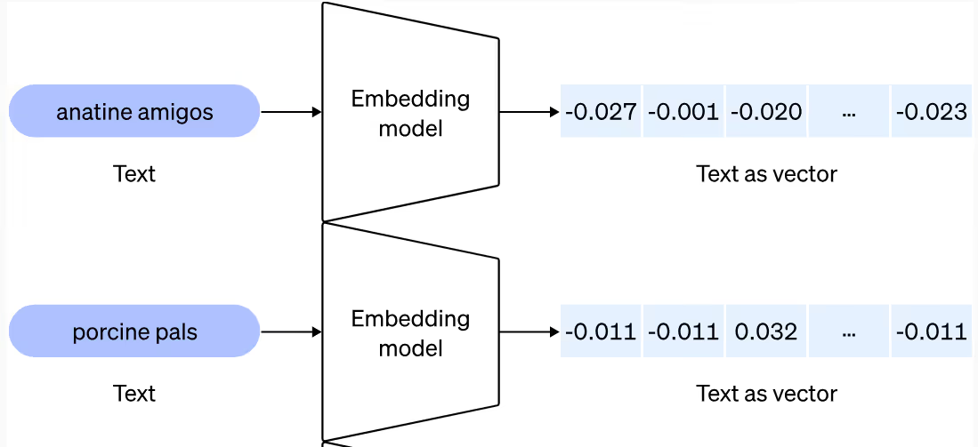
We’ll be using sentence-transformers’ multilingual embeddings for this analysis, but you can definitely experiment with other multilingual embeddings available in the market for this. It maps sentences and paragraphs to a 384-dimensional dense vector space and can be used for tasks like clustering or semantic search. There’s no specific reason behind choosing this model, but I wanted an embedding model that I could use for these four languages (Hindi, English, Spanish, and French), and it turned out it could serve the purpose.

I looked on the internet to see if there was any analysis I could read to understand how different languages behave when it comes to chunking, but sadly I wasn’t able to find one. To understand why we even need such analysis, we need to understand how languages behave, and that’s exactly what we’ll do today. We’ll see how languages behave differently, which confirms that we might need to process texts in different languages separately. Then we’ll move on to trying out chunking approaches on these texts.

The most common approach that people use these days is… I think you can make a guess! It’s RecursiveCharacterTextSplitter(). This analysis will help you understand how different languages behave when we use RecursiveCharacterTextSplitter() in our code and what could be the best chunk size for it. Refer to the code to do it on your text and experiment further.

As we start our analysis, it’s important to know what approaches exist and when to use or avoid them. Overall, the major chunking methods are the following, and we’ll try some of them today:

1. CharacterTextSplitter()
2. TokenTextSplitter()
3. RecursiveCharacterTextSplitter()
4. Semantic Chunking
5. Clustering Based Approaches (CRAG)
6. LLM-based chunking (Agent assisted)

How do you find the best chunk size for RecursiveCharacterTextSplitter()?

Before we understand how languages behave, let’s first see in detail what happens when we use different languages with RecursiveCharacterTextSplitter(), and then we’ll understand why it might be happening in the second section of this blog.

Having seen this myself, I believe that people often use this approach directly while building their projects and then experiment with chunk sizes. I’ve seen people using this in production, so it seems to be the best fit for analyzing fixed character splitting. I analyzed all four languages, and things turned out interesting.

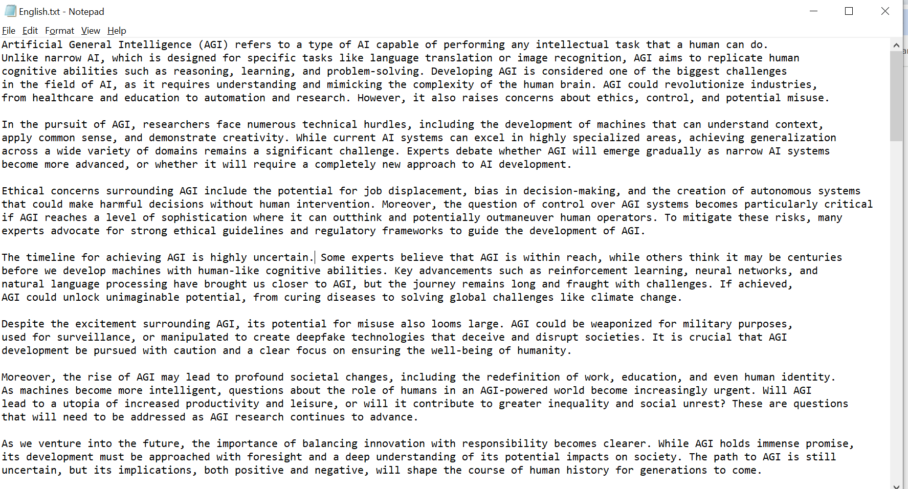
I used different chunk sizes for processing and stored the chunks in LanceDB as vectors, with separate tables per language and chunk size. I used a 50-character overlap for all chunk sizes during this analysis; you can experiment with other overlaps in the notebook.

We can divide the text into chunks and save them into LanceDB using the following code–

import os
from typing import List, Dict, Any, Tuple
from langchain.text_splitter import RecursiveCharacterTextSplitter
from langchain_huggingface.embeddings import HuggingFaceEmbeddings
from langchain.schema import Document
import lancedb
import pandas as pd
from sklearn.metrics.pairwise import cosine_similarity
import nltk

nltk.download('punkt_tab')

def process_text(text: str,
                chunk_sizes: List[int],
                model_name: str = "sentence-transformers/paraphrase-multilingual-MiniLM-L12-v2",
                db_path: str = "/content/lancedb_data",
                language: str = "text") -> Dict:
    
    # Initialize
    embeddings = HuggingFaceEmbeddings(model_name=model_name)
    db = lancedb.connect(db_path)
    processed_data = {}

    # Preprocess text
    text = text.replace("\n", " ")
    for chunk_size in chunk_sizes:
        print(f"\nCreating chunks of size {chunk_size}")

        # Create chunks
        splitter = RecursiveCharacterTextSplitter(
            chunk_size=chunk_size,
            chunk_overlap=50
        )
        chunks = splitter.create_documents([text])
        chunk_texts = [chunk.page_content for chunk in chunks]
        embeddings_list = embeddings.embed_documents(chunk_texts)

        # Store in LanceDB. For each language and for that specific chunk we'll create a single table and store all chunks there.
        table_name = f"{language}_chunks_{chunk_size}"
        df = pd.DataFrame({
            "text": chunk_texts,
            "vector": embeddings_list,
            "chunk_index": range(len(chunks)),
            "char_length": [len(chunk) for chunk in chunk_texts]
        })

        db.create_table(table_name, data=df, mode="overwrite") 
        #table with same name will be overwritten when we rerun the query over another text.

        # Store metadata
        processed_data[chunk_size] = {
            "num_chunks": len(chunks),
            "table_name": table_name,
            "avg_length": df['char_length'].mean()
        }

    return processed_data

The summary of processing English chunks across these four sizes looks like this:

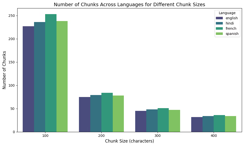
When we used a chunk size of 100, the English text was divided into 227 chunks. As we increase the chunk size, the number of chunks starts reducing, which is expected since more text fits into a single chunk.

But what happens when we process the same text in multiple languages—English, Hindi, French, and Spanish? We processed the same text across all these languages, and the results turned out to be quite interesting.

This pattern changes as we increase the chunk size. When the chunk size increases from 100 to 400, we observe that the difference in the number of chunks becomes less significant with the Recursive Character Text Splitter. English and Hindi texts were split into almost the same number of chunks after a size of 100, while French and Spanish behaved somewhat similarly after 100.

An initial observation is that English and Hindi are quite similar in how they distribute information across chunks. While this isn’t a generalization, similar analyses could be conducted for other languages.

We still can’t choose a chunk size until we test retrieval and see how performance changes with chunk size. Our embedding data is stored in LanceDBm, with corresponding *.lance files for each language and chunk.

Here’s the code to query from tables stored in LanceDB:

def search_chunks(query: str,
                 chunk_size: int,
                 language: str = "text",
                 model_name: str = "sentence-transformers/paraphrase-multilingual-MiniLM-L12-v2",
                 db_path: str = "/content/lancedb_data",
                 top_k: int = 3) -> Dict:

    # Initialize
    embeddings = HuggingFaceEmbeddings(model_name=model_name)
    db = lancedb.connect(db_path)

    # Get query embedding
    print(f"Processing query: '{query}'")
    query_embedding = embeddings.embed_query(query)

    # Search in LanceDB
    table_name = f"{language}_chunks_{chunk_size}"
    table = db.open_table(table_name)
    results = table.search(query_embedding).metric('cosine').limit(top_k).to_pandas()

    # Calculate similarity scores
    similarities = 1 - results['_distance'].values

    # Prepare results
    search_results = {
        'texts': results['text'].tolist(),
        'similarity_scores': similarities.tolist(),
        'char_lengths': results['char_length'].tolist(),
        'query': query,
        'chunk_size': chunk_size,
        'avg_similarity': np.mean(similarities)
    }
    
    return search_results

Refer notebook for implementation.

Before we move on to comparisons, here’s what the result for one chunk size looks like. I searched for the question “एजीआई क्या है?”. For a chunk size of 400 in the Hindi language, we have the following results:

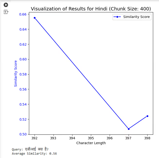
If we examine the combined results for a chunk size of 400 for the same question — “What is AGI?” across all the other languages, they look like this. Note that this plot is based solely on the results for a chunk size of 400. Do you notice anything unusual? Any strange behavior?

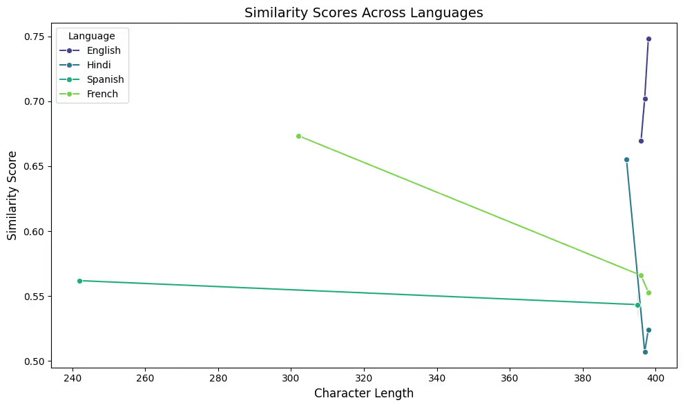
Let’s take a pause and look at the results we got through the retrieval.

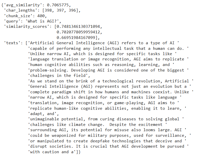
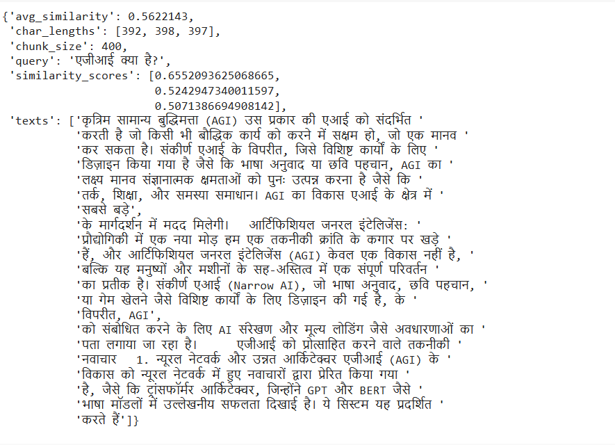
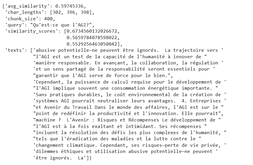
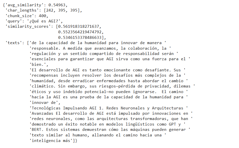
If you look at the retrieved results for chunk size 400, English and Hindi clearly performed better than French and Spanish. Another quick observation from here is that the first retrieved result in the case of correct answers differs greatly from the other two chunks, which do not contain relevant text and are unrelated to the question.

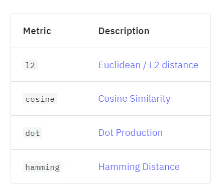
Quick note — We are using the cosine distance metric provided by LanceDB to compare vectors. It also offers other distance metrics that you can use per your use case or experimentation.

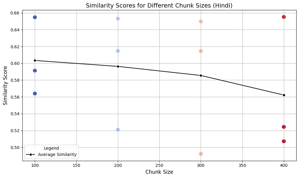
Starting with the Hindi language, for the query — “एजीआई क्या है?”, the similarity scores for multiple chunk sizes look like this:

On the other hand, larger chunks contain more context and information but might not achieve the best average similarity search score.

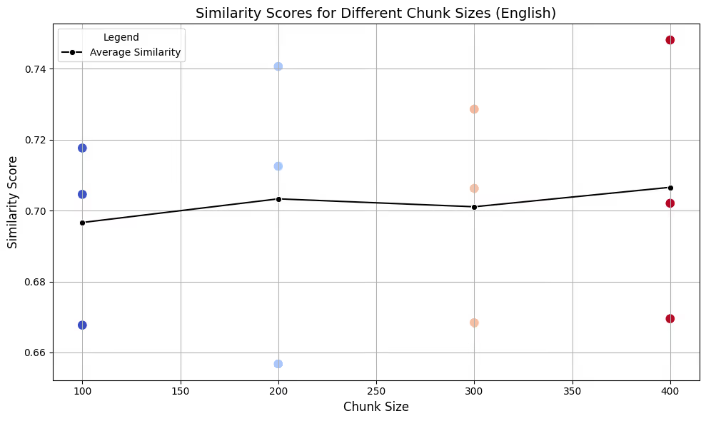
What about English? — look at this chart below.

Now let’s look at the combined plot for all four languages.

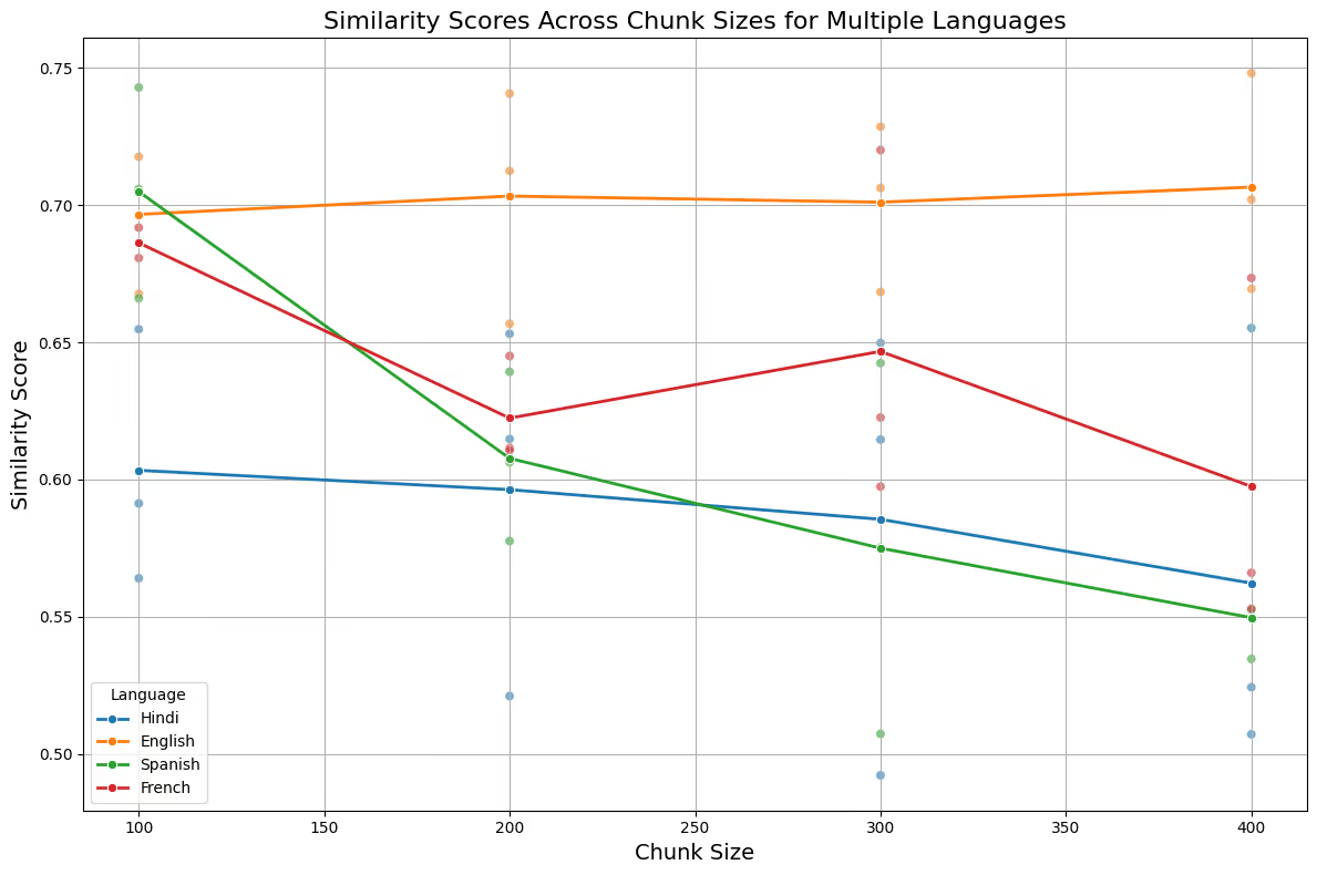
The initial interpretation of this plot shows that we get different results with different chunk sizes for each language. Even though we used the same text and queried on the same chunk sizes, in each language, one chunk size performed better than the others, and there is no direct solution to determine the best size universally.

One clear insight from the above analysis is that, across the four languages processed, Spanish and French behaved differently compared to English and Hindi, both in terms of chunking and retrieval.

Now we can ask why this might be happening and how languages actually differ from each other.

How Languages Behave?

You should understand that language structure, particularly morphology (the study of word formation), plays a crucial role in chunking. Morphology determines how words are formed and how they change to express different meanings, tenses, or cases. This can affect the length and number of chunks, as words in some languages might be more compact or more descriptive than in others.

In our case, if you notice, English and Hindi share certain grammatical structures and sentence patterns that make their chunking behavior more similar. English typically uses a Subject-Verb-Object (SVO) structure, while Hindi often uses a Subject-Object-Verb (SOV) structure. While there are inflections in Hindi, they do not lead to drastically different chunking behavior compared to English.

At the same time, both French and Spanish have more complex morphology compared to English or Hindi, meaning they have a larger number of word forms depending on factors such as gender, number, verb conjugation, and case. These features make chunking and text segmentation different in these languages.

Let’s take an example to understand this better. For the sentence “I eat apples” in English, the subject (“I”) comes first, followed by the verb (“eat”), and then the object (“apples”). This structure is simple and consistent. In Hindi, it would be — “मैं सेब खाता हूँ।”. Here, the subject (“मैं”) comes first, followed by the object (“सेब”), and finally the verb (“खाता हूँ”). The verb is always at the end, which makes it different from English. In French, it’d be — “Je mange des pommes”. French follows the SVO order, just like English. However, when adjectives are involved, they often come after the noun. In Spanish, it’d be — “Yo como manzanas”. Spanish also follows SVO but with some flexibility. Spanish allows dropping the subject (“Yo”), while English, Hindi, and French typically do not.

Note that these (French and Spanish) also follow SVO, but with more frequent adjective-noun inversion and different punctuation rules, which can make chunking different because the chunks may need to account for these structural nuances.

That’s why we need something that not only splits our text using some character limit but also understands the context and what is being talked about. That’s where Semantic Chunking would come into play.

Advanced Chunking: Semantic and Clustering based approach

Limiting chunking to a fixed number of characters often causes loss of information and context between chunks. It rarely makes sense to split text arbitrarily. We need an approach that considers both meaning and context; one such way is semantic chunking.

First, we split the text into individual sentences using (not mandatory) NLTK’s sentence tokenizer. This preserves natural language boundaries rather than breaking text arbitrarily using the number of characters. Here, we can experiment with different models and especially language-specific models available for tokenization.

For example, NLTK provides the option to pass a language as a parameter while splitting into sentences. We’ll use the “sent_tokenize()” function here. It relies on pre-trained language models to determine sentence boundaries. It not only searches for punctuation marks like ‘?’, ‘,’, ‘.’, and ‘!’, but also accounts for abbreviations like “Mr.” and “U.S.A” to make sure these are not interpreted as boundaries, which might happen if you use simple regex code.

There’s another alternative to NLTK, i.e., to use spaCy models. spaCy also provides language-specific tokenizers, and you can definitely experiment with that if you want to.

I tried it on all four languages by passing the language as a parameter and got almost similar results, so I combined approaches for those languages. In Hindi, punctuation is different; instead of full stops (.), it uses “|” (danda). I used sent_tokenize() for all the other three languages and a simple regex splitter for Hindi.

Once we split the larger text into sentences, the next step is to combine these sentences based on semantic similarity to form coherent groups. Two simple strategies are:

1. Sequential Semantic Chunking: Group sentences in order based on similarity. If similarity between the current and next chunk is above a threshold, group them; otherwise, start a new group.
2. Semantic + Clustering: Create embeddings for all sentences, cluster them, and then form chunks by grouping sentences within each cluster. The number of clusters can be chosen programmatically using minimum and maximum chunk size preferences.

Sequential Semantic Chunking

We’ll try both approaches one by one. Starting with the first approach, it’s recommended when the order of content is more important because in this approach, we combine the chunks in sequential order. Ideal use cases could be, for example, if you are processing chat messages, you might want to retain the order of your text.

The high-level flow of semantic chunking would look like this –

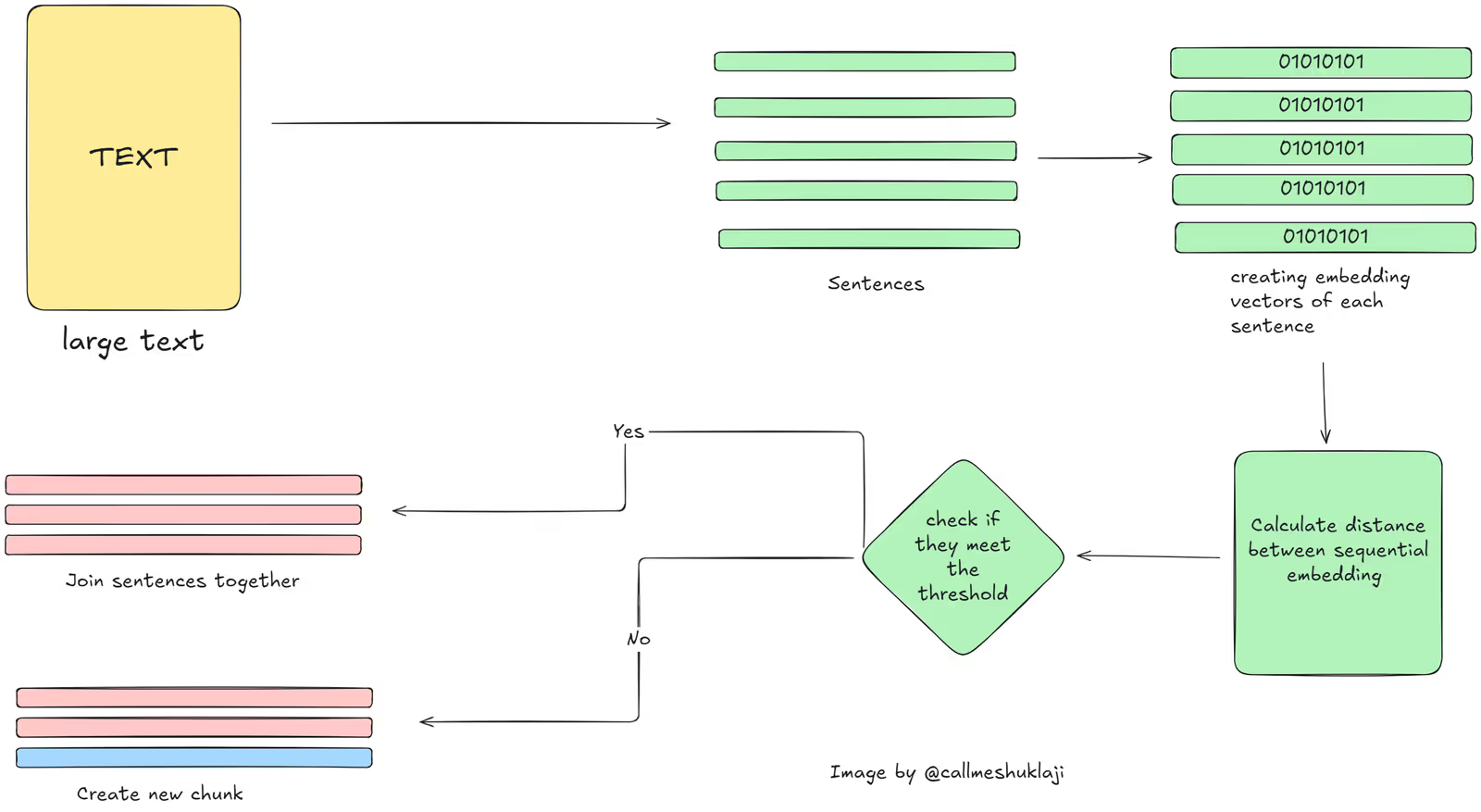
Clearly, we’ll take the text and divide it into sentences. Since there are chances that many sentences will be created during the splitting of the text, we’ll group those sentences in sequence if they are discussing the same topic. Remember those large number of chunks being created when we used fixed character text splitters? Around 200-something, right? What do you think will happen this time? Initially, when we split the text into sentences, we got 90 chunks for English. (Already reduced xd)

Here’s the code snippet that you can refer to for this approach. (use Colab for full code and testing it)–

import re
import numpy as np
from sklearn.metrics.pairwise import cosine_similarity

def store_embeddings(chunks: List[str], table_name: str, model_name: str = "sentence-transformers/paraphrase-multilingual-MiniLM-L12-v2", overwrite=True):
    # Create embeddings
    model = SentenceTransformer(model_name)
    embeddings = model.encode(chunks)

    # Connect to LanceDB
    db = lancedb.connect("./lancedb")

    # If table exists and overwrite is True, recreate it
    
    if table_name in db.table_names() and overwrite:
        db.drop_table(table_name)
    # Create new table
    table = db.create_table(
        table_name,
        data=[{
            "text": chunk,
            "vector": embedding
        } for chunk, embedding in zip(chunks, embeddings)]
    )
    return table

#check colab for full code.

def combine_chunks(chunks: list) -> list:
    for i in range(len(chunks)):
        combined_chunk = ""
        if i > 0:
            combined_chunk += chunks[i - 1]["chunk"]
        combined_chunk += chunks[i]["chunk"]
        if i < len(chunks) - 1:
            combined_chunk += chunks[i + 1]["chunk"]
        chunks[i]["combined_chunk"] = combined_chunk

    return chunks

def add_embeddings_to_chunks(model, chunks: list) -> list:
    combined_chunks_text = [chunk["combined_chunk"] for chunk in chunks]
    chunk_embeddings = model.encode(combined_chunks_text, show_progress_bar=True)
    for i, chunk in enumerate(chunks):
        chunk["embedding"] = chunk_embeddings[i]
    return chunks

def calculate_cosine_distances(chunks: list) -> list:
    distances = []
    for i in range(len(chunks) - 1):
        current_embedding = chunks[i]["embedding"]
        next_embedding = chunks[i + 1]["embedding"]

        similarity = cosine_similarity([current_embedding], [next_embedding])[0][0]
        distance = 1 - similarity

        distances.append(distance)
        chunks[i]["distance_to_next"] = distance

    return distances

To explain a bit about the process going on here – For each pair of consecutive embeddings, the cosine similarity is calculated. Once we get the similarity, we can calculate the distance between each sentence. Then we calculate the threshold value. The threshold is calculated as the percentile value (e.g., the 90th percentile) of the cosine distances. It is essentially a filter to identify “significant transitions” in the text, where the semantic similarity between consecutive sections drops sharply. Then we iterate over the distances and compare each one to the threshold value. If a distance exceeds the threshold, it indicates a significant semantic transition, and its position is added to crossing points.

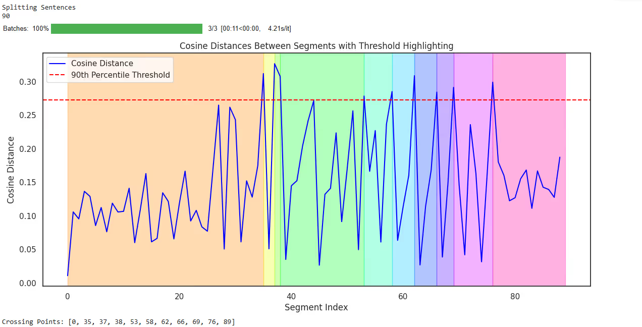
Look at this chart above. Did you notice something? Once we do semantic chunking, we get 11 crossing points, and here we combine similar sentences together. That means these were the points where there was a slight change in context, and other things would have been discussed in the text. For each crossing point, we’ll create a new chunk from there to the next crossing point. This helps in two ways–

1. First, we have reduced the number of chunks drastically.
2. More information related to that specific context is now available in those chunks instead of simply splitting based on character count.

For English, I got 90 sentences initially and 11 chunks of different sizes. A few are very large in size, and a few are small in terms of content, which might be because we started discussing new content in the later part of our text. Still, there are multiple ways to improve the current approach, and it’s important to do so because we might get chunks that are often too large in size, which may create issues later.

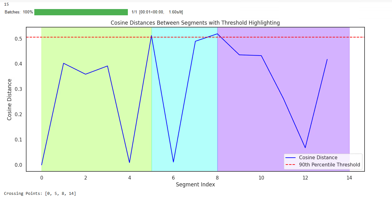
So while this approach made more sense than RecursiveCharacterTextSplitter(), it has its own issues, like very high variance in chunk sizes due to solely matching on the semantics of sentences. That means a few chunks are over 4000 characters long, while some are only 400. The good part of doing this analysis over all the languages is that there’s a similar pattern being observed while processing all of these languages.

They all behaved similarly and had 10-11 chunks at the end, which were far better than many chunks with irrelevant information. The only issue is that we haven’t defined any chunk size limit here. I’ll leave this experimentation to you to create chunks based on both semantics and chunk sizes and then examine the results.

But this approach might not work always. The reason being, what if I started talking about one topic, mixed it with some other topic, and then came back to discussing the same topic again? That means the content should be chunk in such a way that if I ask a certain question about that context, I should get all the details about that particular topic in a chunk, which we might miss due to semantic chunking. What is the solution then? A smart solution would be Clustering-based chunking.

Semantic and Clustering Combined

I read about the clustering-based approach in this paper titled - CRAG .

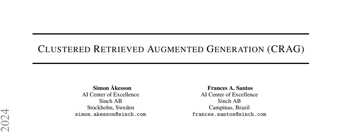
This paper was introduced in May 2024 and provides a detailed insight into how using a clustering-based approach could help you reduce your LLM call costs by reducing the number of tokens being sent.

Logically, there are various ways of doing clustering, and it depends on your use case or type of content. Ideally, if you think about it, there could be infinite ways of doing this, depending on what works and what doesn’t. For example–

1. You can create embeddings of all the text data initially and then create clusters and divide them into chunks. (Does this remind you of any recent paper? Late chunking?)
2. Or you can split your text into sentences and then create clusters on top of their embeddings.
3. Or maybe you can think of other approaches, xd.

I’ll try the second one today. We have the text, we’ll divide it into sentences, and then we’ll use different clustering approaches, with the simplest and most effective one being K-means, and group sentences belonging to similar clusters. That makes sense, right?

A major issue is, that we might need to define the number of chunks as a parameter while using K-means, which we can choose to find programmatically by taking minimum and maximum chunk size preferences as parameters. Another alternative could be trying different clustering approaches like DBSCAN or any other.

Flow in this approach would be like this –

Let’s do it. We’ll first take the text and divide it into sentences. I used the following code depending on the language.

from sentence_transformers import SentenceTransformer
from sklearn.cluster import KMeans
import numpy as np
from typing import List
import nltk
import re
from nltk.tokenize import sent_tokenize

#This is just a part of code. Check notebook for full code for testing.

class SemanticTransformerChunker:
    def __init__(
        self,
        model_name: str = "sentence-transformers/paraphrase-multilingual-MiniLM-L12-v2",
        min_chunk_size: int = 100,
        max_chunk_size: int = 2000,
        threshold_percentile: int = 90
    ):
        
    def determine_optimal_clusters(
        self,
        text_length: int,
        num_sentences: int
    ) -> int:

        """
        Determine optimal number of clusters based on text length
        and desired chunk sizes
        """

        avg_chars_per_sentence = text_length / num_sentences
        min_sentences = max(2, self.min_chunk_size / avg_chars_per_sentence)
        max_sentences = self.max_chunk_size / avg_chars_per_sentence

        return max(2, min(
            num_sentences // 2,  # Don't create too many clusters
            int(num_sentences / min_sentences)  # Ensure minimum chunk size
        ))

    def chunk_text(
        self,
        text: str,
        num_chunks: int = None
    ) -> List[str]:

        # Split into sentences (for those 3 languages)
        sentences = self.split_into_sentences(text)

        if len(sentences) < 3:
            sentences = self.split_hindi_text(text)
            print("splitting hindi text into sentences")

        # Get sentence embeddings
        embeddings = self.get_embeddings(sentences)

        # Determine number of clusters if not provided. it's better to determine this programmatically but we'll see how this might be concerning as well.
        if num_chunks is None:
            num_chunks = self.determine_optimal_clusters(
                len(text),
                len(sentences)
            )

        # Cluster sentences -- #if num_chunks given is more than no. of sentences, we'll take count of sentences as clusters.
        kmeans = KMeans(
            n_clusters=min(num_chunks, len(sentences)),

            random_state=42
        )

        clusters = kmeans.fit_predict(embeddings)
        # Sort sentences by cluster and position
        sentence_clusters = [(sent, cluster, i) for i, (sent, cluster)
                           in enumerate(zip(sentences, clusters))]
        sentence_clusters.sort(key=lambda x: (x[1], x[2]))

        # Combine sentences into chunks
        chunks = []
        current_chunk = []
        current_cluster = sentence_clusters[0][1]

        for sentence, cluster, _ in sentence_clusters:
            if cluster != current_cluster:
                chunks.append(" ".join(current_chunk))
                current_chunk = []
                current_cluster = cluster
            current_chunk.append(sentence)
            
        if current_chunk:
            chunks.append(" ".join(current_chunk))
        return chunks

Initially, we got 87 sentences from our text. After clustering these sentence embeddings, we ended up with 43 clusters for English, which is a reasonable balance. The same analysis on other languages behaved oddly for Hindi but worked decently for French and Spanish.

Now that we have cluster-based chunks, we can check retrieval quality. I saved all the embedding vectors into LanceDB with separate tables per language. I asked three questions to evaluate whether the retrieved chunks made sense. The first five chunks for the question “What is AGI” are:

I believe the first 3-4 chunks contain enough information to answer the question “What is AGI?” On asking a different question, say, “Does AGI control itself?” we got—

This perfectly makes sense since the context is talking about the query being asked.

For each query, the top three chunks contained enough information to answer it. Now let’s look at the final approach before returning to our original questions.

LLM based Chunking

People often call this approach “Agentic Chunking.” As the name suggests, in this approach, we utilize LLMs during the chunking process to create quality chunks, so they can provide better retrieval.

Usually, there are two common approaches:

1. Give the entire text to an LLM and ask it to split into N chunks.
2. Use an LLM to create propositions that add meaning to individual sentences, then chunk those propositions.

The second approach is quite popular these days. You use LLM to create propositions for your sentences. When we do this, the sentences can stand on their own meaning, meaning you don’t necessarily need much context to understand what is being talked about or who the sentence is referring to.

For example, if our text looks like this – “Aman is a good guy. He recently met a boy named Akhil. They started playing chess. Aman liked chess. He plays chess at grandmaster level.”

When we pass this text to the LLM to create propositions, it would come out like this –

[‘Aman is a good guy.’, ‘Aman met a boy named Akhil.’, ‘They started playing chess.’, ‘Aman liked chess.’, ‘Aman plays chess at grandmaster level.’]

Did you notice the second sentence in the lineup? In our text, it was “He recently met a boy named Akhil,” while in the propositions, it turned out to be “Aman met a boy named Akhil,” which does not need surrounding context to understand who is being referred to. I hope you got the point.

Code to create propositions–

from langchain_google_genai import ChatGoogleGenerativeAI
from langchain.prompts import PromptTemplate
from langchain.output_parsers import CommaSeparatedListOutputParser
from typing import List
import google.generativeai as genai
from tqdm import tqdm
from langchain import hub
from langchain.pydantic_v1 import BaseModel

#check colab for full code
def create_propositions(text: str, llm: ChatGoogleGenerativeAI) -> List[str]:
    """Extract propositions from text using Gemini"""
    output_parser = CommaSeparatedListOutputParser()

    try:
        # Get propositions from Gemini
        prompt = get_proposition_prompt(text)
        # prompt = hub.pull("wfh/proposal-indexing")

        response = llm.invoke(prompt)

        response = response.content #make sure you add .content since the response it AI message
        # Parse and clean propositions
        propositions = output_parser.parse(response)
        propositions = [p.strip() for p in propositions if p.strip()]
        return propositions

    except Exception as e:
        print(f"Error processing text: {e}")
        return []

Check Colab for full code

Once we have these propositions, we can follow the same steps as in the semantic or clustering approaches to group them and create the final chunks. However, I wouldn’t recommend this approach for large corpora, as it becomes expensive. Similarly, passing whole documents to LLMs and asking them to return stopping points or chunks directly is rarely cost-efficient.

Still, I’ve included the code to create propositions if you want to try it yourself.

What did we learn?

From our analysis, different languages behave differently when it comes to chunking and retrieval. For some languages, like Hindi, smaller chunk sizes give better precision (which is nearly true for all the languages), while for languages like English, larger chunks (around 400 or more) often work better because they capture more context, improving average retrieval accuracy with RecursiveCharacterTextSplitter().

We also saw how semantic or clustering-based approaches produce better chunks than fixed character splitters. While the high-level approach is similar across languages, sub-steps like sentence splitting need to be language-aware. My recommendation is to copy the notebook, plug in your own text, and see how your language and use case behave.

Clearly, there’s no “one-size-fits-all” formula. If you are using Recursive, you should experiment with chunk sizes. If you are using semantic or clustering-based approaches, you should experiment with parameters like thresholds, number of clusters, and sentence tokenizers.

The choice of embedding model also plays a big role. Multilingual embeddings may treat different languages in different ways, leading to variations in chunking and retrieval. I tried using another embedding model from Sentence Transformers and, while the overall results were similar, the similarity scores differed slightly. There are also strong multilingual models from providers like Cohere that are worth exploring.

There is a trade-off between chunk size and context. Smaller chunks give higher precision but may lose some context, while larger chunks contain more context but may not match as well for retrieval and often contain irrelevant text, which might distract LLMs. You can also store multiple segment lengths within a single database, as we effectively did with semantic chunking by not passing fixed chunk sizes.

Spanish, French, English, and Hindi behaved differently at times and similarly at others. This shows that, beyond context, some languages need special treatment to get the best results. We can look into the specific features of each language, like sentence structure and word formation, and design better preprocessing strategies—especially for languages like Spanish and French. Using language-specific models can help here.

Finally, as much as answer quality depends on chunks, it also depends on the retrieval process. How we store these chunks in vector databases matters a lot. Better indexing and retrieval strategies can improve performance before we even touch the LLM. That’s material for another blog.

Now, coming back to the two questions we asked at the start:

We have different splitters these days, and they are used for different purposes. If you are working on text-only use cases and want a practical way to choose a chunking approach, use the Colab notebook to upload your text files and test it yourself.

Here’s the link to the Colab Notebook .

Key Takeaways

But still, if you are someone looking for a direct answer, I’ll give you a starting point. If you work on –

1. English - If you use RecursiveCharacterTextSplitter() with your application. If you don’t want to use Recursive, use the clustering-based approach directly. It gave the best results and is the most cost-effective approach available.
2. Hindi - I’d not recommend Recursive here unless it’s the worst case and you have no time. For this, try out different text splitters using NLTK or spaCy models and then start with the Semantic Chunk first. If it doesn’t perform well, you can definitely consider clustering-based approaches.
3. French and Spanish - Notice that these languages are kind of similar when compared with English. If you are someone working on them for the first time, go with clustering-based approaches for both of them. They performed very decently.

Overall, I hope this blog has given you a sense of direction to analyze and find the correct chunk size and chunk approach for your language using LanceDB. You can go ahead and experiment further with more questions on the same text or with your own text. Feel free to share your results and findings if you perform further analysis on other languages or different questions.

References

1. Research Papers ,
2. Blogs , and
3. an awesome notebook by Full stack retrieval.