How We Added Geospatial Support To Lance With No New Code

This post is the story of how geospatial data support came to Lance. But here’s what made it remarkable – it required no new code at all, thanks to the Lance format design principles.

It all began with a GitHub discussion. Xin Sun from ByteDance opened a thread about adding geospatial type support to Lance. Instead of writing a proposal asking for someone to implement the feature, Xin showed up with example code snippets demonstrating how to read and write geospatial data in Lance. Points, LineStrings, Polygons, all working out of the box.

How was this possible without any code changes to Lance? The answer lies in its composable foundation that it incorporated from day one: Lance is Arrow-native.

The Power of Arrow-Native Design

Lance as a storage format defines how data is laid out, from a single file (the file format) to multiple files in a table (the table format) to multiple tables in a namespace directory (the namespace format). But all data exchange happens through Apache Arrow in memory. This design choice has profound implications.

Arrow itself is extensible through its extension types . An extension type is a way to give semantic meaning to an underlying Arrow type by attaching metadata. The base type handles the physical representation, while the metadata describes the logical interpretation. Any system that understands Arrow can transport extension types correctly, even without being aware of their semantics.

This is exactly the feature leveraged by GeoArrow , a specification that defines how to store geospatial (geometry and geography) features in Arrow-compatible data structures. It supports the full Simple Feature Access standard: Point, LineString, Polygon, MultiPoint, MultiLineString, MultiPolygon, and GeometryCollection.

How GeoArrow Works

Let’s understand how this works with a concrete example. A 2D point with coordinates (longitude, latitude) needs two float values. In GeoArrow, this is represented as:

• Physical type: A FixedSizeList of 2 Float64 values
• Extension name: geoarrow.point
• Extension metadata: JSON containing coordinate reference system (CRS) information

When you write this data to Lance, it stores the following:

1. The underlying Arrow arrays (the coordinate values)
2. The schema with extension type metadata preserved

When you read it back, Lance reconstructs the Arrow arrays and reattaches the extension metadata. Any GeoArrow-aware library immediately recognizes the column as a Point geometry, not just a list of floats.

import lance
import pyarrow as pa
from geoarrow.rust.core import point, points
import numpy as np

# Create GeoArrow point data
points_2d = points([np.array([1.0, 2.0, 3.0]), np.array([4.0, 5.0, 6.0])])

# Define schema with GeoArrow extension type
schema = pa.schema([
    pa.field(point("xy")).with_name("location")
])

# Write to Lance - no special handling needed
table = pa.Table.from_arrays([points_2d], schema=schema)
ds = lance.write_dataset(table, "s3://bucket/geo-dataset")

# Read back - extension type is preserved
read_table = ds.to_table()
assert read_table.schema.field(0).metadata[b"ARROW:extension:name"] == b"geoarrow.point"

Because Lance faithfully stores Arrow data (including all extension type metadata), any Arrow extension type works in Lance automatically. Points, LineStrings, Polygons, complex geometries with coordinate reference systems – all of it, just works.

Beyond Storage: Geospatial Functions

For stored geospatial data to be useful, you also need to query it by calculating distances, testing intersections and performing spatial joins. This did require us to write some code, but just a few lines.

Lance uses DataFusion as its native Rust query engine. DataFusion provides a powerful, extensible SQL interface for querying Arrow data. And the GeoArrow community has built GeoDataFusion , which extends DataFusion with geospatial functions following the OGC Simple Feature Access standard.

The integration was natural: import GeoDataFusion’s function registry into Lance’s DataFusion context. With this, any user of Lance’s Rust SDK, Python binding, or Java binding can directly invoke geo functions.

import lance
import pyarrow as pa
from geoarrow.rust.core import point, linestring, points, linestrings
import numpy as np

# Create a point at (1, 2)
points_2d = points([np.array([1.0]), np.array([2.0])])

# Create a linestring from (3, 5) to (4, 0)
line_offsets = np.array([0, 2], dtype=np.int32)
linestrings_2d = linestrings(
    [np.array([3.0, 4.0]), np.array([5.0, 0.0])], line_offsets
)

schema = pa.schema([
    pa.field(point("xy")).with_name("point"),
    pa.field(linestring("xy")).with_name("linestring"),
])
table = pa.Table.from_arrays([points_2d, linestrings_2d], schema=schema)
ds = lance.write_dataset(table, "/tmp/geo-sql-demo")

# Query with ST_Distance
batches = (
    ds.sql("SELECT ST_Distance(point, linestring) as dist FROM dataset")
    .build()
    .to_batch_records()
)
print(batches[0].to_pydict())
# {'dist': [2.5495097567963922]}

The full SQL interface supports functions like ST_Distance, ST_Intersects, ST_Contains, ST_Within, ST_GeomFromText, and many more. No special configuration is required; the functions are available as soon as you use Lance’s SDKs.

Accelerating Geospatial Queries: The R-Tree Index

Geospatial functions alone aren’t enough for production workloads. Scanning every row to check ST_Intersects on a billion-row dataset would be prohibitively slow. We need spatial indexing.

Driven by their use cases, the Lance community really stepped up here. There were long discussions about the best approach for spatial indexing, and this is one of those rare situations where we had the bandwidth to thoroughly evaluate all the potential options.

As one of the most active groups in the Lance community, Uber had significant interest in geospatial support and was eager to help, which is not surprising considering all the Uber cars we see on the road. Jay Narale provided an implementation of a geo index using a BKD tree, based on the approach in Apache Lucene.

Meanwhile, Xin Sun from ByteDance provided an alternative implementation using an R-Tree so we could compare the two approaches side-by-side. We ran extensive performance comparisons across different data distributions, query patterns, and dataset sizes. In the end, the R-Tree approach proved to be the better fit for Lance’s workload characteristics, and that’s what was ultimately shipped.

How the R-Tree Index Works

The R-Tree index in Lance is a static, immutable 2D spatial index built on bounding boxes. It’s designed as a multi-level hierarchical structure:

• Leaf pages store tuples of (bbox, rowid) for indexed geometries
• Branch pages aggregate child bounding boxes and store pageid pointers to child pages
• A single root page encloses the entire tree

The index uses a packed-build strategy with Hilbert curve sorting to maximize spatial locality. Hilbert sorting imposes a linear order on 2D items using a space-filling curve, ensuring that geometries close in space are also close in storage. This dramatically improves the effectiveness of bounding box pruning during queries.

Why R-Tree Works Well for Lance

R-Trees are known for delivering excellent query performance, but they come with a tradeoff: they are difficult to update efficiently. Inserting or deleting geometries can trigger cascading rebalancing operations that degrade performance.

For Lance, this tradeoff is actually a perfect fit. Lance stores indexes in object storage, and at the point of storage the index is already immutable. When new data arrives, Lance doesn’t perform inline index updates. Instead, indexes are updated asynchronously through retraining, which rebuilds the index to incorporate new geometries. This aligns with Lance’s broader philosophy of treating indexes as derived artifacts that can be regenerated from the source data.

The immutable nature of stored indexes also enables some nice properties: indexes can be cached aggressively, read in parallel without coordination, and versioned alongside the data they index. The “limitation” of R-Tree mutability becomes irrelevant when your storage model is already designed around immutability.

For the full specification of how R-Tree indexes are stored in Lance, see the R-Tree Index Specification .

Visualizing R-Tree Pruning

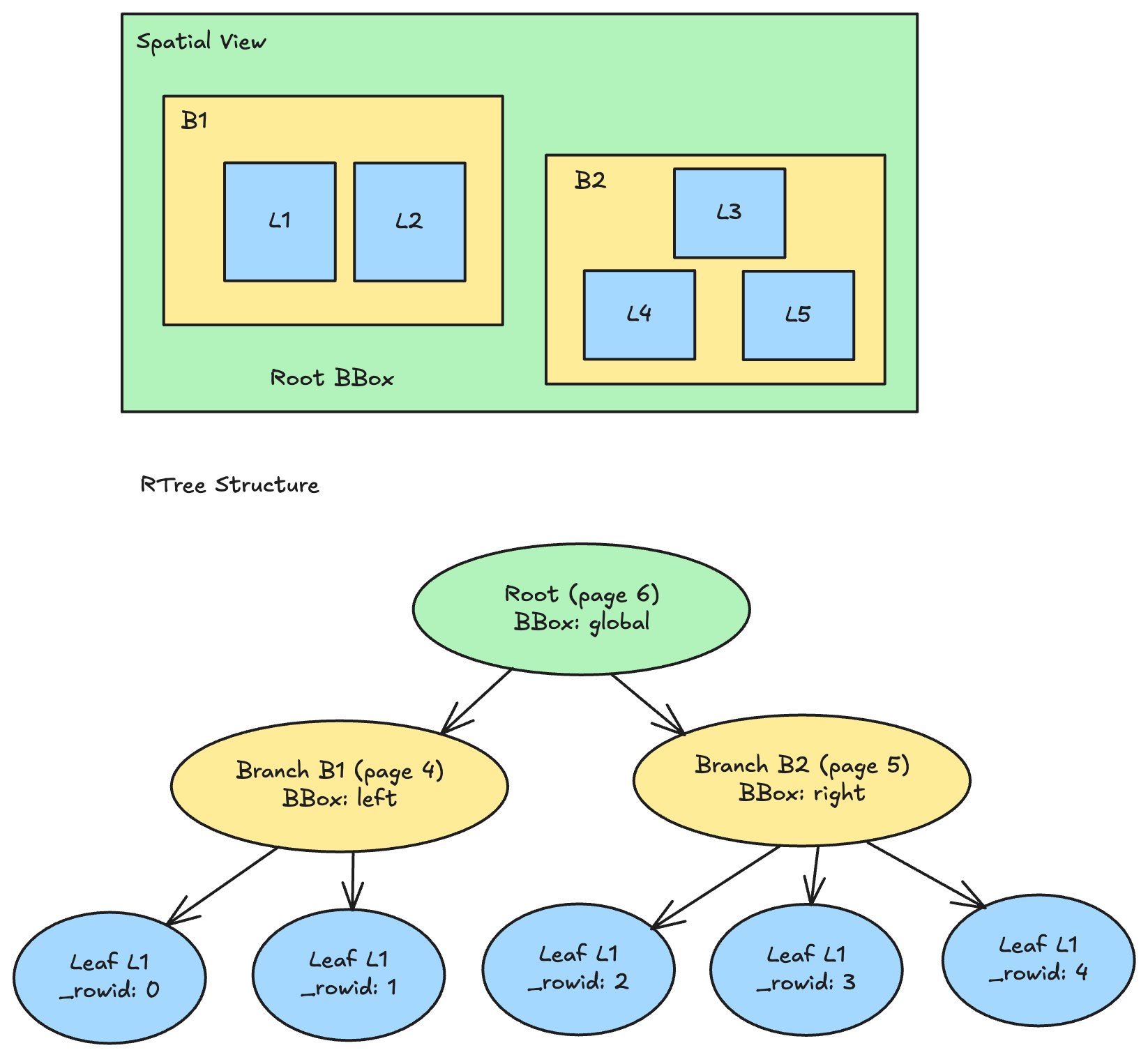
For a filter ST_Intersects(geometry, query_bbox), it:

1. Starts at root → query_bbox intersects root? Yes → descend
2. Checks B1 → intersects? No → prune entire subtree (skip L1, L2)
3. Checks B2 → intersects? Yes → descend
4. Checks L3, L4, L5 → only L4 intersects → return row 3 as a candidate

Once we have the candidate row IDs, readers can leverage Lance’s random access capability to efficiently access the right rows in the right files to get other requested column data.

Using R-Tree Index with pylance

When you create an R-Tree index and run a spatial query:

import lance
import pyarrow as pa
from geoarrow.rust.core import linestring, linestrings
import numpy as np

# Create 10,000 random linestrings
num_lines = 10000
line_offsets = np.arange(num_lines + 1, dtype=np.int32) * 2
linestrings_2d = linestrings(
    [np.random.randn(num_lines * 2) * 100, np.random.randn(num_lines * 2) * 100],
    line_offsets,
)

schema = pa.schema([
    pa.field("id", pa.int64()),
    pa.field(linestring("xy")).with_name("geometry"),
])
table = pa.Table.from_arrays(
    [np.arange(num_lines, dtype=np.int64), linestrings_2d], schema=schema
)
ds = lance.write_dataset(table, "/tmp/rtree-demo")

# Create the R-Tree index
ds.create_scalar_index("geometry", "RTREE")

# Query with index acceleration
sql = """
SELECT id, geometry
FROM dataset
WHERE ST_Intersects(geometry, ST_GeomFromText('LINESTRING (2 0, 0 2)'))
"""

# Check the query plan to verify index usage
plan = ds.sql(sql).build().explain_plan()
print(plan)
# LanceRead: uri=/tmp/rtree-demo, projection=[id, geometry], ...
#   ScalarIndexQuery: query=[Intersect(geometry ...)]@geometry_idx
#   ^^^^^^^^^^^^^^^^^^^^^^^^^^^^^^^^^^^^^^^^^^^^^^^^^^^^^^^^^^^
#   R-Tree index is being used for spatial filtering

results = ds.sql(sql).build().to_batch_records()

The index accelerates a wide range of spatial predicates:

All these queries use bounding box filtering to prune candidates, with exact geometry verification performed by the execution engine on the remaining rows. The result is orders of magnitude faster spatial queries on large datasets.

Comparison with Other Formats

How does Lance’s approach compare to other geospatial solutions? Recently, the Apache Parquet community published a great blog post explaining how Parquet supports geospatial types. It’s worth reading for context on how the broader ecosystem approached this. Below, I’ll highlight three key architectural differences in Lance’s approach.

Native GeoArrow vs. WKB Encoding

Parquet’s native geospatial support introduces GEOMETRY and GEOGRAPHY logical types, storing geometries in Well-Known Binary (WKB) encoding. WKB is a standard binary serialization that’s widely supported across GIS tools, making it an excellent choice for interoperability with the existing geospatial ecosystem.

Lance takes a different approach, storing geometries in the types defined by the GeoArrow extension type specification. For a Point, that means a FixedSizeList of two Float64 coordinates rather than a binary blob. This reflects Lance’s Arrow-native architecture: Arrow extension types are preserved end-to-end for seamless data exchange.

These are different design choices driven by different priorities.

WKB in Parquet optimizes for maximum compatibility with existing GIS tools. Any system that understands WKB can immediately work with the data. The format is self-describing and well-standardized, and it provides a smooth transition path for users migrating from GeoParquet to the official Parquet geospatial types.

GeoArrow in Lance optimizes for native columnar access, achieving better read write performance and compression since values are stored in typed columnar arrays and structs rather than rows of WKB blobs. Arrow-native compute engines can work directly with the coordinate arrays, while non-Arrow engines can use GeoArrow libraries to convert at read or write time. This approach aligns with Lance’s Arrow-native architecture and delegates the right amount of responsibility to the GeoArrow library rather than reimplementing geospatial encoding in Lance.

In the end, both formats chose the direction that fit their architecture most naturally, and both formats work with GeoArrow as the common interchange layer. For Parquet, engines that want columnar coordinate access can use GeoArrow libraries to parse WKB. For Lance, engines that only consume WKB can use GeoArrow libraries to convert at read time:

import lance
import pyarrow.parquet as pq
from geoarrow.rust.core import to_wkb, from_wkb

# Read WKB from Parquet, convert to GeoArrow
parquet_table = pq.read_table("s3://geo-data.parquet")
geoarrow_array = from_wkb(parquet_table.column("geometry"))

# Read GeoArrow from Lance, convert to WKB
lance_table = lance.dataset("s3://bucket/geo-dataset.lance").to_table()
wkb_array = to_wkb(lance_table.column("geometry"))

Secondary Index vs. Column Statistics

Parquet’s geospatial support includes storing bounding box statistics in row group metadata. Each row group records the minimum and maximum extents of the geometries it contains, enabling row group pruning at query time.

Lance does not store statistics about bounding boxes in column metadata. Instead, we delegate this entirely to the R-Tree index. This follows the same index-first strategy we apply to all data types: for example, we also don’t provide direct column statistics and bloom filters in file metadata, but we provide zone maps, bloom filters, and other secondary indexes.

Each approach has tradeoffs. Column statistics are always available without extra setup and add minimal overhead, making them good for ad-hoc queries where you haven’t pre-optimized. A dedicated index like R-Tree requires explicit creation but can provide more sophisticated pruning for complex spatial predicates.

Unified Format vs. Layered Architecture

Parquet is a file format that integrates with table formats like Apache Iceberg and Delta Lake. Each layer has its own type system: Parquet defines both physical and logical types, while Iceberg and Delta define their own logical types that map onto Parquet’s type system. On top of that, each query engine (Spark, Trino, DuckDB, etc.) implements its own mapping to both the table format and Parquet at the metadata and data processing layers. Geospatial support requires coordination across all these layers.

Lance is both a file format and a table format. Lance schema closely resembles the Arrow schema for maximum compatibility, and all data exchange happens through Arrow. Geospatial types are defined once and work consistently whether you’re reading a single file or querying a multi-file dataset. Engines mainly work with Arrow types and Arrow data to integrate Lance, and require no knowledge of Lance internals.

This reflects different ecosystem philosophies. The Parquet approach enables mix-and-match: you can use Parquet with Iceberg, Delta, Hive, or raw files, each with their own type semantics. While you can also use the Lance file format with other table formats, the main goal for Lance is the simplicity of one format, one schema specification, consistent behavior everywhere, in order to provide an end-to-end multimodal lakehouse format layer.

Putting it Together: Geospatial Modality in the Multimodal Lakehouse

Geospatial data support is a natural fit for the Multimodal Lakehouse – location data often accompanies images, sensor readings, and other rich media, alongside traditional tabular data. With Lance’s unified support for geospatial types, vector embeddings, and SQL queries, you can express powerful multimodal retrieval patterns in a single query.

The use case below is quite common: it combines geospatial filtering with vector similarity search, which is a perfect use case for Lance.

Find all images taken within 1 km of this location that are similar to this reference image."

import lance
import pyarrow as pa
import numpy as np
from geoarrow.rust.core import point, points

# Assume we have a dataset with images, their embeddings, and capture locations
# Schema: id, image_embedding (vector), location (geoarrow.point)

ds = lance.dataset("s3://bucket/image-dataset")

# Reference location (e.g., Times Square)
ref_lat, ref_lon = 40.758, -73.9855

# Reference image embedding (from your embedding model)
ref_embedding = get_embedding(reference_image)  # 512-dim vector

# Find similar images within 1km of Times Square
# ST_DWithin filters by distance, then vector search ranks by similarity
results = (
    ds.scanner(
        filter=f"ST_DWithin(location, ST_Point({ref_lon}, {ref_lat}), 1000)",
        prefilter=True,
    )
    .nearest("image_embedding", ref_embedding, k=10)
    .to_table()
)

The R-Tree index prunes locations outside the 1 km radius, and the vector index finds the most similar images among the remaining candidates. Both indexes work together, each accelerating its respective modality.

Acknowledgments

This work is a testament to what organic open source collaboration can achieve. Without any top-down coordination, contributors from ByteDance, Uber, the Apache DataFusion community, the GeoArrow community independently found their way to Lance and came together to make performant geospatial support a reality.

Xin Sun from ByteDance kickstarted the entire effort by demonstrating what was already possible with Lance’s Arrow-native design, then contributed the R-Tree implementation and the lance-geo crate that we ultimately shipped.

Jay Narale from Uber contributed the alternative BKD tree implementation and ran exhaustive benchmarks comparing both approaches to help us find the optimal solution.

A huge thanks to the broader Apache DataFusion, GeoDataFusion and GeoArrow communities. Kyle Barron , one of the original creators of GeoArrow and GeoDataFusion, provided tremendous guidance throughout the integration. Tim Saucer helped navigate the DataFusion ecosystem. And of course, Will Jones from LanceDB coordinated across the three repositories to ensure proper dependency management and version compatibility.

Future Work

While geo support in Lance is now production-ready, there’s more we want to do:

1. Geospatial Lance datasets on HuggingFace. With HuggingFace Lance integration now available, it’s the perfect time to start converting geospatial datasets to Lance. There are many excellent datasets listed on geoarrow.org/data and beyond. We’re looking forward to the community leveraging this powerful combination of HuggingFace and Lance to share and access geospatial data at scale.

2. Lakehouse engine integrations. Today, geo functions and indexing work through Lance’s SDK interface. We want to extend this support to other Lance connectors like lance-spark , lance-trino , lance-duckdb and lance-ray . The heavy lifting has already been done by the Lance SDK, GeoArrow and GeoDataFusion. Engine integration is really the last mile to map engine semantics to GeoArrow and GeoDataFusion semantics. We’d encourage anyone interested in contributing to give it a try!

3. Pluggable secondary index system. Geospatial support brings significant dependencies (geo libraries, spatial algorithms, R-Tree implementation). We want to make our secondary index system pluggable so users who don’t need geo capabilities don’t have to include these dependencies. This is part of a broader effort to keep Lance’s core lean while supporting specialized workloads.

We’re excited about where this integration may be used, because it demonstrates what’s possible when you build on solid foundations. Arrow-native design, extensible query engines, and an engaged community can deliver capabilities that feel like magic. If you’re looking to integrate Lance into your lakehouse, let us know what you’d like to see via our discussions page on GitHub, and ask your questions on Discord !