Make your SQL Workflows Multimodal With LanceDB × DuckDB

Prashanth Rao

•

May 22, 2026

•

Engineering

Table of Contents

This is a title

This is a subtitle

The typical enterprise data stack relies on different tools for different workloads: DuckDB is commonly used by developers to run analytical queries in SQL, and LanceDB is common for multimodal storage and fast search. Real user queries may span across both systems, with search, joins and aggregations regularly occuring in the same query.

The LanceDB team recently collaborated with the DuckDB team to release the Lance extension as a core extension, bringing the two ecosystems closer. This post discusses a hands-on walkthrough that demonstrates the extension in practice. But first, more on the underlying problem this solves.

More glue code means more drift

Analytical queries (involving joins, aggregations, ad-hoc filters) are normally written in SQL. Multimodal questions (vector search over text and image embeddings, retrieval across a corpus of product images) benefit from LanceDB's native storage and retrieval patterns for this kind of data. When someone asks "how many customers purchased beige shoes with floral patterns?", the answer involves querying over multiple tables from different sources. If embeddings, image bytes and metadata don't live in one place, there's a cost to maintaining more glue code to keep everything in sync and retrieve them from multiple sources.

There's also a quieter and more significant cost: drift. In many traditional stacks, image bytes, embeddings, and metadata live in three different systems and evolve on three different cadences. The consequences (e.g., embeddings that retrieve the wrong product, joins on item IDs that no longer exist, indexes built against bytes that have since been replaced) only surface at query time. Keeping multimodal data co-located with embeddings and metadata, and versioned together, removes that whole class of problem.

The Lance extension in DuckDB allows you to query any Lance table from DuckDB directly: scans, vector search, joins to other DuckDB tables, aggregation, and writing results back, using the same, familiar DuckDB interface. DuckDB users can query Lance vector or full-text search indexes with normal SQL while Lance handles the expensive ANN search, filtering, and reranking close to the data, returning only the relevant results to DuckDB.

The Dataset

Let's make the workflow concrete with the Amazon Berkeley Objects (ABO) dataset. It's a good fit for this walkthrough because it looks like the kind of mixed data that shows up in real applications: product records come with structured metadata, descriptive text, and associated images. Together those three streams make it a genuinely multimodal product dataset. ABO has ~145K items in total, but for this walkthrough, we ingest a 5K-product subset to keep it lean. The same workflow scales unchanged to the full dataset.

The multimodal blobs (images) naturally go into LanceDB along with the rest of the metadata. Everything for one product (normalized metadata, the raw image bytes, and the embeddings) lives in a single row of a Lance table. The columns are also rich enough, and carry unique identifiers, that they join cleanly to other DuckDB tables downstream.

Co-locating the modalities also means they get governed together, via dataset versioning. Metadata, image bytes, embedding vectors, and any indexes Lance builds over them all live under the same table version, so a collaborator pulling version N gets exactly the bytes, embeddings, and indexes that were used in this run, enhancing reproducibility.

In the products Lance table, each row carries normalized fields such as title, brand, product_type, material, style, and category_path. It also carries the raw image bytes in an image_bytes column (a binary type, more on this below), plus a local image_path for reference. On top of these we add three derived columns that make the table useful for search: fts_text for keyword search, multimodal_vec for CLIP-based cross-modal retrieval, and text_vec for text-semantic search with intfloat/multilingual-e5-base.

Let's proceed to build a multimodal product catalog in LanceDB first.

Step 1: Build the Product Catalog in LanceDB

Download the ABO dataset from official source. The first step is to turn the raw dataset into a LanceDB table. To do this, we open a connection to a LanceDB directory and create a named products table.

import lancedb

db = lancedb.connect("./abo-products-lance")

From there, the preprocessing flow is mostly about shaping the data for the retrieval stage. We read the ABO listings, match each product to its corresponding image, and normalize the nested multilingual metadata into plain string columns such as title, brand, material, and category_path. The image embeddings come from a Hugging Face CLIP model, giving us a cross-modal retrieval signal. The text embeddings come from the intfloat/multilingual-e5-base SentenceTransformer model, giving us a text-semantic view over the description of the product. The result is a single products table that keeps metadata, image references, and vectors together in one place.

The full PyArrow schema of the LanceDB table is shown below:

import pyarrow as pa

schema = pa.schema(
    [
        pa.field("item_id", pa.string()),
        pa.field("title", pa.string()),
        pa.field("description", pa.string()),
        pa.field("brand", pa.string()),
        pa.field("product_type", pa.string()),
        pa.field("category_path", pa.string()),
        pa.field("material", pa.string()),
        pa.field("color", pa.string()),
        pa.field("style", pa.string()),
        pa.field("image_path", pa.string()),
        pa.field("image_bytes", pa.large_binary()),
        pa.field("fts_text", pa.string()),
        pa.field("multimodal_vec", pa.list_(pa.float32(), multimodal_dim)),
        pa.field("text_vec", pa.list_(pa.float32(), text_dim)),
    ]
)

The image_bytes column is the part that pulls the image store inside the catalog. It's a regular Arrow large_binary column: Lance writes the bytes into the same columnar table as the metadata and embeddings, and DuckDB exposes them as ordinary SQL BLOBs. We'll see exactly what that buys us in Step 5.

Prior to ingestion, we have raw source data scattered across multiple directories. After the ingestion step, we have a LanceDB-managed catalog with a table name and a schema that's ready for both search and analytics.

Step 2: Scan the Catalog in DuckDB

With the lance extension, DuckDB can scan the Lance-backed table directly, which means we can seamlessly move from data preparation to querying it via SQL without copying the dataset into a separate relational system first.

It's simple to install and load the lance extension in a DuckDB CLI:

INSTALL lance;
LOAD lance;

The simplest way to scan the table is by directly pointing DuckDB to the local LanceDB directory.

SELECT item_id, title, brand, product_type, image_path
FROM './abo-products-lance/products.lance'
LIMIT 5;

That is already enough to inspect the catalog and confirm that the rows look the way we expect. We can see the product identifiers, the normalized metadata, and the image path all coming back through ordinary SQL.

For day-to-day work and scaling usage across a larger team, attaching the catalog via a namespace is recommended, as it's cleaner and more reusable than carrying around raw file paths. DuckDB lets us attach the LanceDB directory as a namespace:

ATTACH './abo-products-lance' AS abo (TYPE LANCE);

This makes the tables accessible via the abo namespace. The query now looks a lot cleaner.

SELECT item_id, title, brand, category_path
FROM abo.main.products
LIMIT 5;

_💡_{What is "main" in the schema?}_{‍
In DuckDB, the "main" table or default schema is called}_main_{. When you create a table without specifying a schema, it's automatically placed in this main schema within the opened DuckDB database.}

Namespaces matter in a practical way for developers. They give DuckDB a clear view over the Lance-backed tables you attach, and they make the SQL easier to read once the workflow grows beyond one quick scan. Instead of thinking in terms of "some path on disk that happens to contain a Lance table," we can treat the catalog as something named and queryable inside DuckDB, just as we would do inside LanceDB.

That may sound like a small shift, but it makes the rest of the workflow much easier to follow. Once the table is attached, we can stop thinking about storage details and start asking more interesting questions of the data. Next, we'll create a small DuckDB sales table so we can join it to the catalog during retrieval.

Step 3: Create DuckDB Table

Once the catalog is attached, it becomes easy to mix it with other tables that DuckDB can materialize or scan. A realistic example is customer or sales data that may live somewhere else, such as Postgres. DuckDB is very good at pulling those kinds of tables into a local analytical workflow and joining them to data coming from other formats.

For this walkthrough, let's keep it simple. We'll create a small local DuckDB database representing sales events, where each record has its own id plus an item_id that points back to a product in the LanceDB catalog.

First, open the DuckDB database and attach the Lance namespace so the product catalog is available inside the same connection:

import duckdb
import random

random.seed(23)
SALES_ROW_LIMIT = 1000

con = duckdb.connect("./sales.duckdb")
con.execute("INSTALL lance")
con.execute("LOAD lance")
con.execute("ATTACH './abo-products-lance' AS abo (TYPE LANCE)")

With that connection in place, we can pull the shoe product IDs from the attached Lance table and use them to create the local DuckDB sales table:

shoe_ids = [
    row[0]
    for row in con.execute(
        """
        SELECT item_id
        FROM abo.main.products
        WHERE product_type = 'SHOES'
        """
    ).fetchall()
]

sales_rows = [(i, random.choice(shoe_ids)) for i in range(1, SALES_ROW_LIMIT + 1)]

con.execute("CREATE TABLE sales (id INTEGER, item_id VARCHAR)")
con.executemany("INSERT INTO sales VALUES (?, ?)", sales_rows)

SALES_ROW_LIMIT controls how many synthetic sales rows we generate in DuckDB. The script is run with SALES_ROW_LIMIT = 1000 to keep this demo lightweight, but you can imagine a typical sales table going into the millions of rows quickly.

In a real deployment, you wouldn't generate this table by hand. The same sales rows would more likely live in Postgres, Snowflake, or as Parquet files on S3, and DuckDB has first-class extensions for pulling each of those into the same query. The local table here is a stand-in: anywhere DuckDB can reach a relational table, the rest of this walkthrough applies unchanged.

Before doing any join, we can inspect the table on its own and confirm that it's just a small local DuckDB database whose main table contains a surrogate key and a product key:

┌─────┬────────────┐
│ id  ┆ item_id    │
│ --- ┆ ---        │
│ i32 ┆ str        │
╞═════╪════════════╡
│ 1   ┆ B06X9FMB85 │
│ 2   ┆ B07T3LV191 │
│ 3   ┆ B07MWW4CVX │
└─────┴────────────┘

The table simply tells us what customer id purchased what product item_id.

Step 4: Retrieval Pipeline

Now we can connect the two tools into a more realistic retrieval flow. Imagine a user asks a natural-language question such as, "which customers purchased beige shoes with floral patterns?". In a real application, an agent might break that question down before retrieval happens. We won't build that full agent loop here, but it's enough to assume that the agent has decomposed the question to the image-oriented concept beige shoes floral patterns.

This is a more elaborate retrieval problem than it looks at first glance. "Beige" is something you might recover from a color column with simple keyword search: if the column is populated, if the seller spelled it that way, if the catalog isn't multilingual. "Floral patterns" is squarely a visual concept: many products with floral patterns don't say so in their text fields, and many that do say so use different words ("flower," "embroidery," "print"). The benefit of searching against an image embedding space is that the model can "see" the pattern even when the metadata doesn't describe it.

With the Lance extension, this retrieval doesn't require stepping out of DuckDB. We compute a CLIP query vector in Python, pass it into lance_vector_search(...), and treat the top-k results as an ordinary relation inside SQL.

Here's a Python snippet that shows the image embedding workflow via CLIP:

import duckdb
import torch
from typing import Any
from transformers import CLIPModel, CLIPProcessor

image_keywords = "beige shoes floral patterns"

clip_model = CLIPModel.from_pretrained("openai/clip-vit-base-patch32")
clip_processor: Any = CLIPProcessor.from_pretrained("openai/clip-vit-base-patch32")

clip_inputs = clip_processor(
    text=[image_keywords],
    return_tensors="pt",
    padding=True,
    truncation=True,
)

def _as_embedding_tensor(vectors) -> torch.Tensor:
    if isinstance(vectors, torch.Tensor):
        return vectors
    for attr in ("image_embeds", "text_embeds", "pooler_output", "last_hidden_state"):
        value = getattr(vectors, attr, None)
        if isinstance(value, torch.Tensor):
            if attr == "last_hidden_state":
                return value[:, 0, :]
            return value
    raise TypeError(f"Unsupported embedding output type: {type(vectors)!r}")

with torch.no_grad():
    clip_query_vec = clip_model.get_text_features(**clip_inputs)
    clip_query_vec = _as_embedding_tensor(clip_query_vec)
    clip_query_vec = torch.nn.functional.normalize(clip_query_vec, dim=-1)
    clip_query_vec = clip_query_vec.squeeze().to(torch.float32).cpu().tolist()

The retrieval pipeline is shown below. DuckDB runs the top-k vector search over the attached Lance table, then immediately joins those retrieved products to the sales table (which is a DuckDB table). The output is much closer to the original user question, because it joins sales rows in DuckDB with the product metadata retrieved from Lance.

con = duckdb.connect("sales.duckdb")
con.execute("INSTALL lance")
con.execute("LOAD lance")
con.execute("ATTACH './abo-products-lance' AS abo (TYPE LANCE)")

result = con.execute(
    """
    WITH top_products AS (
      -- Retrieve the top-3 nearest products from Lance, restricted to shoes.
      SELECT item_id, title, brand, color, _distance
      FROM lance_vector_search(
        'abo.main.products',
        'multimodal_vec',
        ?,
        k = 3,
        prefilter = true
      )
      WHERE product_type = 'SHOES'
    )
    -- Join the retrieved Lance rows to the DuckDB sales table and aggregate
    -- to one row per matched product, with how many sales it drove.
    SELECT
      p.item_id,
      p.title,
      p.brand,
      p.color,
      p._distance,
      count(*) AS purchase_count
    FROM sales s
    JOIN top_products p USING (item_id)
    GROUP BY ALL
    ORDER BY p._distance ASC
    """,
    [clip_query_vec],
).pl()

┌────────────┬────────────────────────────┬───────────────┬───────────────────────┬───────────┬────────────────┐
│ item_id    ┆ title                      ┆ brand         ┆ color                 ┆ _distance ┆ purchase_count │
│ ---        ┆ ---                        ┆ ---           ┆ ---                   ┆ ---       ┆ ---            │
│ str        ┆ str                        ┆ str           ┆ str                   ┆ f32       ┆ i64            │
╞════════════╪════════════════════════════╪═══════════════╪═══════════════════════╪═══════════╪════════════════╡
│ B072JTL1HX ┆ Red Wagon Girls' Slip on…  ┆ Red Wagon     ┆ Multicolor Red Floral ┆ 1.388191  ┆ 3              │
│ B07JQC1FSV ┆ Jenny Rhodos 2252778…      ┆ Jenny         ┆                       ┆ 1.395716  ┆ 2              │
│ B08CHP4X9R ┆ Amazon Essentials Zapat…   ┆ Amazon Essen. ┆                       ┆ 1.409938  ┆ 2              │
└────────────┴────────────────────────────┴───────────────┴───────────────────────┴───────────┴────────────────┘

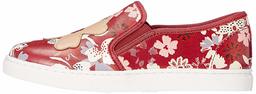
There are 3 products, with 7 total purchases between them. The interesting one is the second row: a beige mocassin with a laser-cut floral pattern, where the color field is blank and neither the title nor the description contains the word "floral." A keyword query on color = 'beige' or description LIKE '%floral%' would have missed it entirely. The image embedding picked it up, because that's where the floral pattern actually lives: in the pixels, not in the text.

Once we have the joined result, follow-up analytical questions are easy to express in SQL. For example, if the next question by a human or an agent is "how many customers purchased beige shoes with floral patterns?", we can aggregate directly on top of the same table:

count_result = con.execute(
    """
    WITH top_products AS (
      SELECT item_id, _distance
      FROM lance_vector_search(
        'abo.main.products',
        'multimodal_vec',
        ?,
        k = 3,
        prefilter = true
      )
      WHERE product_type = 'SHOES'
    )
    SELECT count(*) AS num_customers_beige_floral_shoes
    FROM sales s
    JOIN top_products p USING (item_id)
    """,
    [clip_query_vec],
).pl()

# Returns a count of 7.

Retrieval from image similarity, text similarity, or metadata stops being a special case. It becomes another part of the query plan, one that can be exposed as tools for agents. It's natural to keep extending the analysis with joins, counts, aggregates, and whatever other SQL questions the application needs to answer next.

Materializing results back into LanceDB

Once a retrieved slice becomes useful, there is no reason to leave it as an ephemeral query result. DuckDB can materialize it straight back into the attached LanceDB catalog using CREATE TABLE in the attached namespace. This is a good reminder that the Lance extension in DuckDB is not just a read-only integration: it also lets DuckDB write results back into LanceDB.

con.execute(
    """
    CREATE OR REPLACE TABLE abo.main.beige_floral_shoe_candidates AS
    WITH top_products AS (
      SELECT item_id, title, brand, color, product_type, _distance
      FROM lance_vector_search(
        'abo.main.products',
        'multimodal_vec',
        ?,
        k = 3,
        prefilter = true
      )
      WHERE product_type = 'SHOES'
    )
    SELECT
      p.item_id, p.title, p.brand, p.color, p._distance,
      count(*) AS purchase_count
    FROM top_products p
    JOIN sales s USING (item_id)
    GROUP BY ALL
    """,
    [clip_query_vec],
)

After this runs, the attached namespace contains both the original products table and a derived beige_floral_shoe_candidates table produced from joined retrieval and sales analysis. Namespaces keep these related tables clean and easy to discover as the dataset grows.

Step 5: Image Bytes Returned Directly from SQL

This is where keeping multimodal data natively stored in the storage layer pays off. Everything so far could, in principle, work against a DuckDB or Lance table that only stored pointer URLs: even a vector DB and an object store glued together would do roughly the same job. The next step below is more interesting: direct image retrieval from SQL, in the same result set as the metadata, with no separate fetch step.

Recall that the schema includes an image_bytes column of type large_binary(). Lance stores those bytes in the same columnar table as the metadata and the embeddings, and DuckDB's Lance extension surfaces them as ordinary SQL BLOB. That means a single SELECT can hand the caller everything needed to render or process the matching product, without leaving the SQL session.

Let's try a different query than "beige shoes". We'll search for "colorful floral slip-on shoes":

floral_keywords = "colorful floral slip-on shoes"

clip_inputs = clip_processor(
    text=[floral_keywords],
    return_tensors="pt",
    padding=True,
    truncation=True,
)

with torch.no_grad():
    floral_query_vec = clip_model.get_text_features(**clip_inputs)
    floral_query_vec = _as_embedding_tensor(floral_query_vec)
    floral_query_vec = torch.nn.functional.normalize(floral_query_vec, dim=-1)
    floral_query_vec = floral_query_vec.squeeze().to(torch.float32).cpu().tolist()

Now a pure vector search (no join, no sales table), selecting image_bytes straight from the catalog. We also project octet_length(image_bytes) so we can see the bytes are real before we render them:

floral_result = con.execute(
    """
    SELECT
      item_id,
      title,
      color,
      octet_length(image_bytes) AS num_bytes,
      image_bytes,
      _distance
    FROM lance_vector_search(
      'abo.main.products',
      'multimodal_vec',
      ?,
      k = 5,
      prefilter = true
    )
    WHERE product_type = 'SHOES'
    ORDER BY _distance ASC
    """,
    [floral_query_vec],
).pl()

┌────────────┬───────────────────┬──────────────────┬───────────┬──────────────────┬───────────┐
│ item_id    ┆ title             ┆ color            ┆ num_bytes ┆ image_bytes      ┆ _distance │
│ ---        ┆ ---               ┆ ---              ┆ ---       ┆ ---              ┆ ---       │
│ str        ┆ str               ┆ str              ┆ i64       ┆ binary           ┆ f32       │
╞════════════╪═══════════════════╪══════════════════╪═══════════╪══════════════════╪═══════════╡
│ B072JTL1HX ┆ Red Wagon Girls'  ┆ Multicolor Red   ┆ 5781      ┆ b"\xff\xd8\xff\x ┆ 1.40058   │
│            ┆ Slip on Skate…    ┆ Floral           ┆           ┆ e0\x00\x10JFIF…  ┆           │
│ B079W2J9CV ┆ Amazon Brand -    ┆                  ┆ 7629      ┆ b"\xff\xd8\xff\x ┆ 1.433998  │
│            ┆ Symbol Men's Lo…  ┆                  ┆           ┆ e0\x00\x10JFIF…  ┆           │
│ B01MTEI8M6 ┆ The Fix Amazon    ┆ Havana Tan       ┆ 6225      ┆ b"\xff\xd8\xff\x ┆ 1.457601  │
│            ┆ Brand Women's F…  ┆                  ┆           ┆ e0\x00\x10JFIF…  ┆           │
│ B08248X7RJ ┆ The Drop Zapatos  ┆ Rosado/Rojo      ┆ 3312      ┆ b"\xff\xd8\xff\x ┆ 1.485661  │
│            ┆ Mule Puntiagu…    ┆                  ┆           ┆ e0\x00\x10JFIF…  ┆           │
│ B074F16RLC ┆ Amazon Brand -    ┆ Red              ┆ 5081      ┆ b"\xff\xd8\xff\x ┆ 1.494503  │
│            ┆ Symbol Men's Re…  ┆                  ┆           ┆ e0\x00\x10JFIF…  ┆           │
└────────────┴───────────────────┴──────────────────┴───────────┴──────────────────┴───────────┘

The num_bytes column shows that each result carries a real binary payload: between roughly 3KB and 8KB of JPEG data per row. We can hand the raw image_bytes straight to anything that wants them. Writing the top result to a local directory is simple:

top_row = floral_result.row(0, named=True)
out_path = Path(f"{top_row['item_id']}.jpg")
out_path.write_bytes(top_row["image_bytes"])

That produces a valid JPEG file, byte-identical to the source.

Top result: A red and white floral slip-on skate sneaker

One SQL query returned the ranked neighbors, the metadata, and the image bytes together. No object-store fetch, no path resolution, no glue layer between the catalog and the consumer: the bytes are just a column, and retrieving an image looks like retrieving a string or numerical metadata.

This has implications on downstream code simplicity and performance. Exposing the results via an API can stream the bytes to a client, a notebook can render the image inline, and a training pipeline can grab the retrieved slice as one Arrow table with the images already attached. None of those consumers needs to know where the images "really" live.

Why This Combination Works

If you're a data practitioner working with diverse multimodal datasets, here are the key takeaways from this post:

Native multimodal storage with versioning. LanceDB stores metadata, embeddings, and the image bytes themselves, in one place. Versioning and data evolution features baked in.
One query interface in SQL, including vector search. DuckDB attaches the Lance table via a namespace and runs scans, filters, vector search, aggregations or joins to other DuckDB or Lance tables, without leaving the SQL session.
Read and write data on the fly The Lance extension isn't read-only. DuckDB can materialize derived results back into LanceDB, turning ad-hoc analyses into reusable tables that you can persist in your storage layer of choice.
No glue layer between bytes and queries. A single SELECT returns ranked retrieval results with the image bytes attached. The downstream consumer (UI, API, notebook, training pipeline, or LLM agent that can issue SQL) gets everything in one round trip.

If you want to try the full walkthrough, inspect the code, or adapt the examples to your own dataset, the companion repo is here. For more on the extension itself, see the Lance extension docs in DuckDB and the lance-duckdb repo, and let us know if you have feature requests.

Attribution

This walkthrough uses the Amazon Berkeley Objects dataset, licensed under CC BY 4.0. All credit for the data, including the images, belongs to Amazon.com, and to the creators of the original dataset.