Your object detection model in an autonomous vehicle training job just failed a deployment test because it struggles on specific edge cases (like pedestrians at a distance). Even though you have frames from thousands of hours of dashcam footage already sitting in object-storage, getting the right frames into a clean training split and into your DataLoader might take you a whole week.
It shouldn't have to be that way.
The bottleneck here isn't compute — it's everything that happens between training runs:
- Finding the right data, deriving the right features, deduplicating near-identical frames, creating reproducible splits, and doing it again when new footage arrives.
- A new feature idea triggers a full dataset rewrite.
- A new data source triggers a migration.
- And when you finally make it to training, your H100 spends more time waiting on data than running matrix multiplications.
The core problem is that traditional ML data stacks were never designed for fast iteration on large-scale AI datasets. They were fine when models were trained once or twice a quarter, but not when you're trying to close failure-mode gaps on a weekly cadence. This is especially true when working with multimodal data at petabyte-scale. In a traditional stack that consists of an object store, an annotation database, preprocessing scripts, feature store/VectorDB and CSV manifests, every intermediate step tends to require maintaining a separate system with its own failure mode.
LanceDB is designed to address these problems faced by ML engineers and researchers, at large scale. It's an AI-native multimodal lakehouse built on Lance, an open-source columnar format designed around ML access patterns. This post walks through an end-to-end AV perception pipeline. Each stage uses the same LanceDB table and its features for ingestion, curation, evolution and training without any intermediate file format or hand-off between systems, allowing you to move from raw data to trained models in hours, not weeks.
The experiment setup
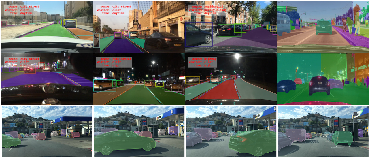
We'll use BAIR's BDD100K dataset as a smaller representation of real-world AV dashcam footage dataset. It involves curating three deployment-critical failure modes, deduplicating with vector search, and training Faster R-CNN (an object detection model), using LanceDB as the single data layer at every stage. The goal is to show what the iteration cycle looks like when the data layer is designed for it: new feature idea to query result in minutes, new footage to updated training split in four commands, checkpoint to reproducible data snapshot with a version number.
Autonomous vehicle perception models fail in predictable ways. For example, let's say your COCO-pretrained Faster R-CNN degrades on three deployment-critical scenarios that are underrepresented in standard benchmarks:
The fix is targeted fine-tuning on curated slices. But curating the right data across these three modes requires different signals from different places. In a conventional stack, those signals live in separate systems: annotation databases, metadata stores, preprocessing scripts.
LanceDB based workflow overview
┌─ Fleet footage (BDD100K, ~100k dashcam frames)
│
│                          │ Ingest
│                          ▼
│  ┌───────────────────────────────────────────────────────────┐
│  │                    bdd100k  [Lance table]                 │
│  │  image_bytes · weather · scene · timeofday · timestamp    │
│  │  ann_categories · ann_bboxes · ann_occluded · split       │
│  │  ┌──────────────────────────────────────────────────────┐ │
│  │  │  Blob storage     — fast reads, no object-store hop  │ │
│  │  │  Multimodal       — bytes + structs + vectors        │ │
│  │  │  Stable row IDs   — incremental view refresh         │ │
│  │  └──────────────────────────────────────────────────────┘ │
│  └───────────────────────────────────────────────────────────┘
│                          │
│                          │ backfill_geneva.py  (Geneva UDFs — incremental, checkpointed)
│                          │
│                          │  Tier 1 — CPU:  has_person · has_rider · scene_description
│                          │  Tier 2 — GPU:  person_bbox_area_pct  (Faster R-CNN)
│                          │               clip_embedding [512-d]  (CLIP ViT-B/32, IVF-PQ)
│                          │  Tier 3 — GPU:  dhash [64-bit]  (dHash) + IVF L2 → is_duplicate
│                          │
│                          │  ┌──────────────────────────────────────────────────────┐
│                          │  │  Zero-copy evolution  — new column, no table rewrite │
│                          │  │  Incremental backfill — only calculate for new rows  │
│                          │  │  Checkpointed         — crash-safe, restart mid-run  │
│                          │  │  Ray-distributed      — scales to thousands of nodes │
│                          │  └──────────────────────────────────────────────────────┘
│                          │
│                          │  EDA & curate
│                          │  ┌──────────────────────────────────────────────────────┐
│                          │  │  SQL         — columnar index, no JOIN, no export    │
│                          │  │  FTS         — BM25 on scene_description             │
│                          │  │  CLIP vector — text→image · image→image · discovery  │
│                          │  │  Hybrid      — CLIP + SQL pre-filter, single query   │
│                          │  └──────────────────────────────────────────────────────┘
│                          │
│                          │  (Materialized views)
│                          │  ┌─ Views ──────────────────────────────────────────────┐
│                          │  │  Living SQL queries — curation filter in one place   │
│                          │  │  Versioned refresh  — table.version links weights→data│
│                          │  └──────────────────────────────────────────────────────┘
│                          │
│              ┌───────────┼──────────────┐
│              ▼           ▼              ▼
│    bdd100k_rider  bdd100k_nighttime  bdd100k_distant
│    _{train,val}   _person_{t,v}      _person_{t,v}
│    [Materialized  [Materialized      [Materialized
│       view]          view]              view]
│              └───────────┼──────────────┘
│                          │
│                          │
│                          │  ┌─ Training ──────────────────────────────────────────┐
│                          │  │  Permutation API — random-access over Lance, no copy │
│                          │  │  PyTorch DataLoaders — direct from Lance tables      │
│                          │  │  High GPU utilization (MFU) — reads direct from Lance│
│                          │  └──────────────────────────────────────────────────────┘
│                          ▼
│               ┌──────────────────┐
│               │    Checkpoint    │  ← version = exact data snapshot
│               │ + table.version  │
│               └──────────┬───────┘
│                          │ new footage arrives
│               ┌──────────▼────────────────────────────────────┐
│               │  append → backfill (new rows only)             │
│               │  → refresh views → train again                 │
└───────────────┴───────────────────────────────────────────────┘
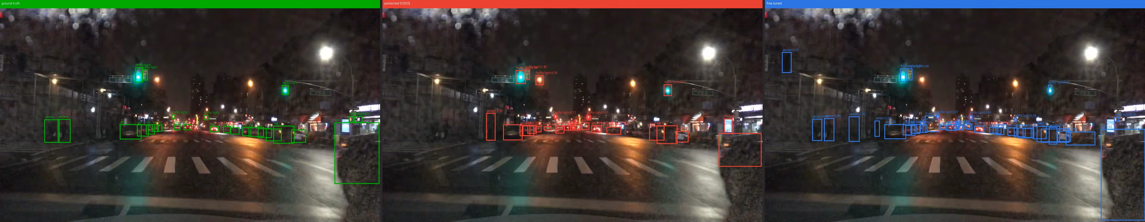
Sample results after training
Green = ground truth · Red = COCO pretrained baseline · Blue = fine-tuned model
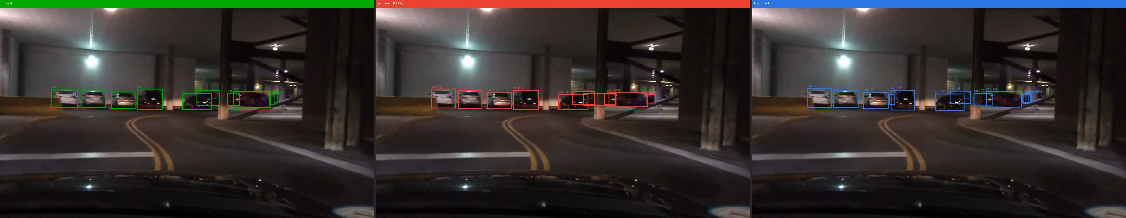
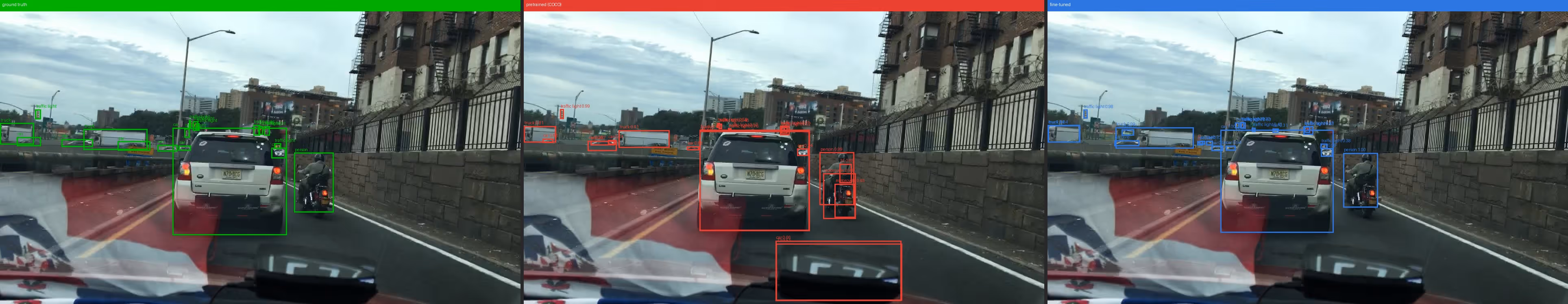
2. Fine-tuned model makes no false predictions for the rider
3. Fine-tuned model is able to correctly detect distant people in the dark (extreme left) while base model can't
Workflow
Native Multimodal support: 100k BDD100K frames land in a single Lance table with raw JPEG bytes, weather strings, annotation lists, and split labels all in one schema. That table is the only data artifact the rest of the pipeline reads from or writes to. No separate image store, no external vector database and no annotation database to manage.
Zero-copy schema evolution: Derived signals like has_person, has_rider, etc., are added as new columns in bdd100k without duplicating any existing data.
Feature engineering at scale: Each derived column is computed by a Geneva UDF, which is a Python function or class that Geneva distributes across workers, writing results back to LanceDB table. It is checkpointed, meaning a crash at frame 70,000 of 80,000 resumes from the last checkpoint, not frame zero. The same UDF that runs on a laptop runs on a cluster of hundreds of machines with zero code changes.
Advanced retrieval and filters: SQL, BM25 full-text search, and vector search are all first-class index types on different columns of the same table. FTS on scene_description finds rare scenarios via natural language keywords. The clip_embedding vector index enables text-to-image and image-to-image search for exploratory data analysis (EDA). SQL filters on fields like timeofday, has_person etc., allow finding edge cases like wrong or missing annotations.
Materialized views: Training splits like bdd100k_rider_train or bdd100k_nighttime_person_train are named tables in LanceDB, defined by a SQL WHERE clause, not CSV exports. When new footage arrives, mv.refresh() appends only rows that satisfy the filter. As a result, this is incremental: nothing is rebuilt from scratch.
Built-in versioning Every add(), backfill(), and refresh() increments the table version. Training scripts log table.version alongside every checkpoint, a permanent link between weights and the exact data snapshot that produced them, with no external versioning system.
Permutation API and native PyTorch support Faster R-CNN trains directly against each materialized view via the Permutation API, a dataloading utility of LanceDB and reads go straight to training loop, allowing you to hit peak MFU in your training jobs. No copy, no intermediate format.
Detailed Walkthrough
Ingestion
Structured multimodal table from unstructured data
The BDD100K dataset comes as separate zip file for each split of images, and each type of annotation in JSON files. Something like this:
bdd100k/
  ├── images/
  │   ├── 100k/
  │   │   ├── train/          # 70,000 JPEGs
  │   │   │   ├── 0000f77c-6257be58.jpg
  │   │   │   └── ... (70k files)
  │   │   ├── val/            # 10,000 JPEGs
  │   │   └── test/           # 20,000 JPEGs (no labels)
  │   ├── 10k/
  │   │   ├── train/          # subset for segmentation tasks
  │   └── seg/
  │
  ├── labels/
  │   ├── det_20/
  │   │   ├── det_train.json  # single JSON for all 70k train frames
  │   │   └── det_val.json    # single JSON for all 10k val frames
  │   ├── pan_seg/
  │   └── sem_seg/
This is just a subset of labels. There's other type of task labels and video clips available in the dataset. With LanceDB, you can turn this unstructured, multi-folder dataset into a table with strict schema containing multimodal data blobs inline.
The full schema for the Lance table mixes types that would normally require separate storage systems:
BDD_SCHEMA = pa.schema([
    pa.field("image_bytes", pa.large_binary()),           # raw JPEG — Lance blob storage
    pa.field("weather",     pa.string()),
    pa.field("timeofday",   pa.string()),
    pa.field("ann_categories",  pa.list_(pa.string())),   # parallel lists per bbox
    pa.field("ann_bboxes",      pa.list_(pa.list_(pa.float32()))),
    # ... more annotation fields ...
])
LanceDB allows you to define table schemas in both PyArrow and Pydantic formats.
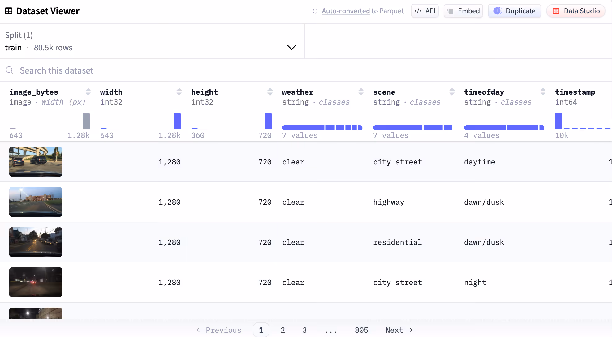
💡 LanceDB <> Hugging Face integration
You can upload any LanceDB dataset to Hugging Face to automatically enable rich table viewer and other HF-datasets native features, like streaming.
Here's the link to the full enriched dataset artifact generated from this workflow, and uploaded to huggingface-hub
Feature Engineering
Geneva UDFs for data evolution
The conventional approach to feature engineering has a structural problem, that it's not incremental. Every new feature requires running the whole script again. If it crashes at frame 70,000 of 80,000, you restart at frame 0.
With Geneva, you just wrap your transformation functions as UDFs, which are Python functions decorated with @udf. The backfill operation creates a distributed job to run the UDF, populating the column values in your LanceDB table, with checkpoints that show progress every N rows. The table evolves with new features, with zero-copy.
Below, we show some UDFs that we used in this workflow:
Simple annotation-derived UDFs (CPU based, no image decoding):
Here's a couple examples of a very simple features, that create new features in the table based on the already existing annotation feature column:
@udf(data_type=pa.bool_(), input_columns=["ann_categories"])
def has_person(ann_categories) -> bool:
    return "person" in list(ann_categories)

@udf(data_type=pa.string(), input_columns=["weather", "scene", "timeofday"])
def scene_description(weather, scene, timeofday) -> str:
    return f"{timeofday} {weather} scene on a {scene}"
GPU inference UDFs
When there's processing and setup required for a task like model loading, you can use batched and/or stateful UDFs. You can create a setup function in the class and invoke in __call__. It runs on workers and loads the model lazily on first invocation, then reuses it for every subsequent batch:
@udf(data_type=pa.float32(), input_columns=["image_bytes", "width", "height"], num_gpus=1, cuda=True)
class PersonBboxAreaPct:
    def __init__(self):
        self.model = None          # not loaded here — driver has no GPU

    def _load_model(self):
        self.model = load_detector().cuda()   # once per worker, reused across batches

    def __call__(self, image_bytes, width, height) -> pa.Array:
        if self.model is None:
            self._load_model()
        predictions = self.model(decode_images(image_bytes))
        return pa.array([bbox_area_pct(pred, w, h) for pred, w, h in zip(predictions, width, height)])
person_bbox_area_pct is the critical signal for the "distant pedestrian" failure mode: frames where a person annotation exists but occupies less than 20-30% of the frame are exactly the hard cases — distant, small figures the pretrained model is more likely to miss.
💡 UDF
For BDD100K, which ships with ground-truth boxes, this could be computed directly fromann_bboxesas a fast CPU UDF. The Faster-RCNN UDF models a production scenario: raw, unlabeled fleet footage where no ground truth exists and a detector is the only way to measure pedestrian prominence. The Geneva backfill pattern, UDF registered as a column is incrementally computed and immediately queryable in SQL.
Running the backfill
job_id = tbl.backfill(
    "person_bbox_area_pct",
    udf=PersonBboxAreaPct(),
    concurrency=4,        # parallel workers (1 per GPU for GPU UDFs)
    checkpoint_size=32,   # commit progress every N fragments — safe to interrupt
)
The concurrency parameter can be set from 1 (local run on a laptop) to hundreds, that run on a KubeRay cluster. checkpoint_size makes the job crash-safe: a restart picks up from the last committed checkpoint, not frame zero.
After all backfills complete, every derived signal sits as a flat, queryable column alongside the original ingested fields. No joins, no manifests. We generate many features using Geneva in this workflow, including the ResNet18 embeddings and is_duplicate flag which we will use in next section.
Curation
Explore and gather insights from large scale multimodal datasets
With LanceDB, you can run SQL, full-text search, and vector search on the same table, allowing you to explore and run analysis on massive tables without having to materialize everything in memory.
With all signals as new features, the entire curation workflow is splitting dataset using SQL filters, which LanceDB supports natively:
# Total rows in train split - 80,000
tbl.count_rows(filter="timeofday = 'night' AND has_person = true")
# → 6,431 frames

tbl.count_rows(filter="has_person = true AND person_bbox_area_pct < 30.0")
# → ~3,200 frames where a person is annotated but occupies less than 30% of the frame
The scene_description column — generated by a Geneva UDF from the frame's weather, scene, and time-of-day attributes — gets an FTS index. Researchers can then iterate on rare-scenario queries in natural language without needing to write SQL predicates:
tbl.create_fts_index("scene_description")
tbl.search("rainy night pedestrian intersection", query_type="fts").limit(10).to_pandas()
Deduplication via vector search: Although BDD100K is dashcam footage dataset, it's highly curated and smaller in size, so it doesn't have many duplicates. But in real world there can be many duplicates in the dataset as consecutive frames within a clip are nearly identical pixels and training on them wastes compute and over-represents specific road segments. The dedup pipeline follows the exact same Geneva backfill pattern:
1. DHash UDF — backfill dhash: a 64-bit perceptual hash per frame, stored as a vector oftype list<float32>[64].
2. Build an IVF index on dhash.
3. is_duplicate UDF — backfill is_duplicate: for each row, find the nearest non-self neighbour via vector search; flag as duplicate if Hamming distance ≤ threshold (like 5,10).
# is_duplicate is now just a boolean column — filter it like anything else
tbl.count_rows(filter="has_rider = true AND split = 'train' AND is_duplicate = false")
The hash, the vector index, and the duplicate flag all live on bdd100k. The materialized views that follow automatically apply the dedup filter to training splits.
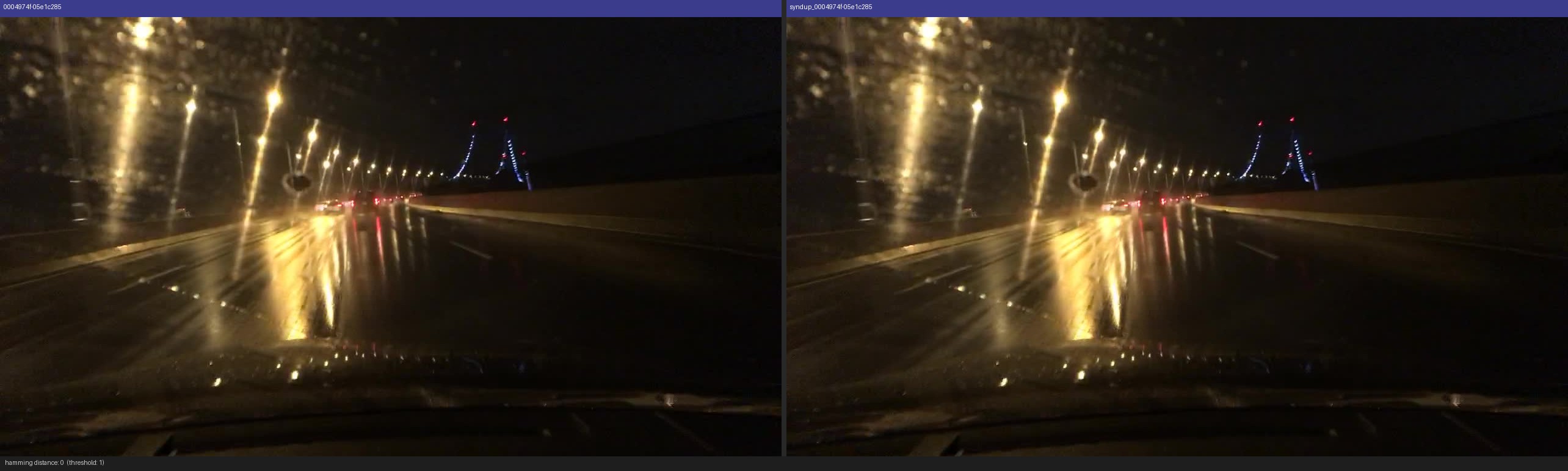
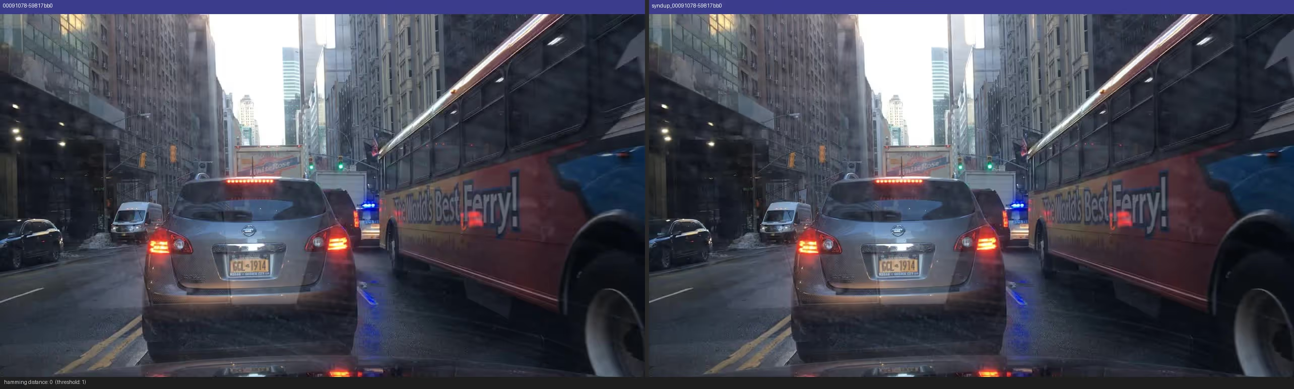
To validate the pipeline end-to-end, we append 1,000 exact-copy rows back into the table (new image_id, same image_bytes) and confirm that every injected row is flagged is_duplicate = true at Hamming distance 1 — a ground-truth test
Example duplicates plotted by the visualization helper from the project repo.
CLIP vector search for EDA: SQL and FTS work well when you know what you're looking for. But failure-mode discovery is inherently open-ended. You want to find frames you can't describe with a SQL predicate. That's where the clip_embedding column comes in: a 512-dimension embedding backfilled by a Geneva GPU UDF, with a cosine IVF-PQ index built after backfill. Because CLIP's image and text encoders share the same embedding space, every query that works as text also works as an image.
Text → Image : Retrieve frames matching a natural-language description. SQL can filter timeofday = 'night', but can't express "a small person barely visible in the distance." CLIP embeddings, however, can.
vec = encode_text("a person far away walking on a dark road at night") # or other queries

tbl.search(vec, vector_column_name="clip_embedding").metric("cosine").limit(8).to_pandas()
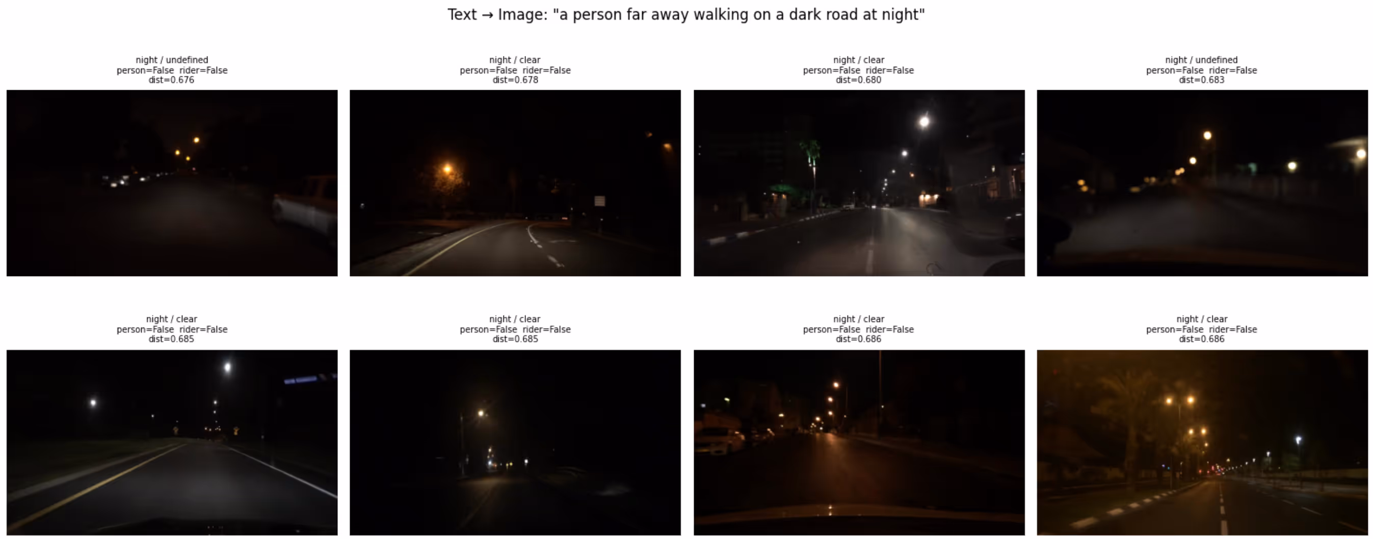
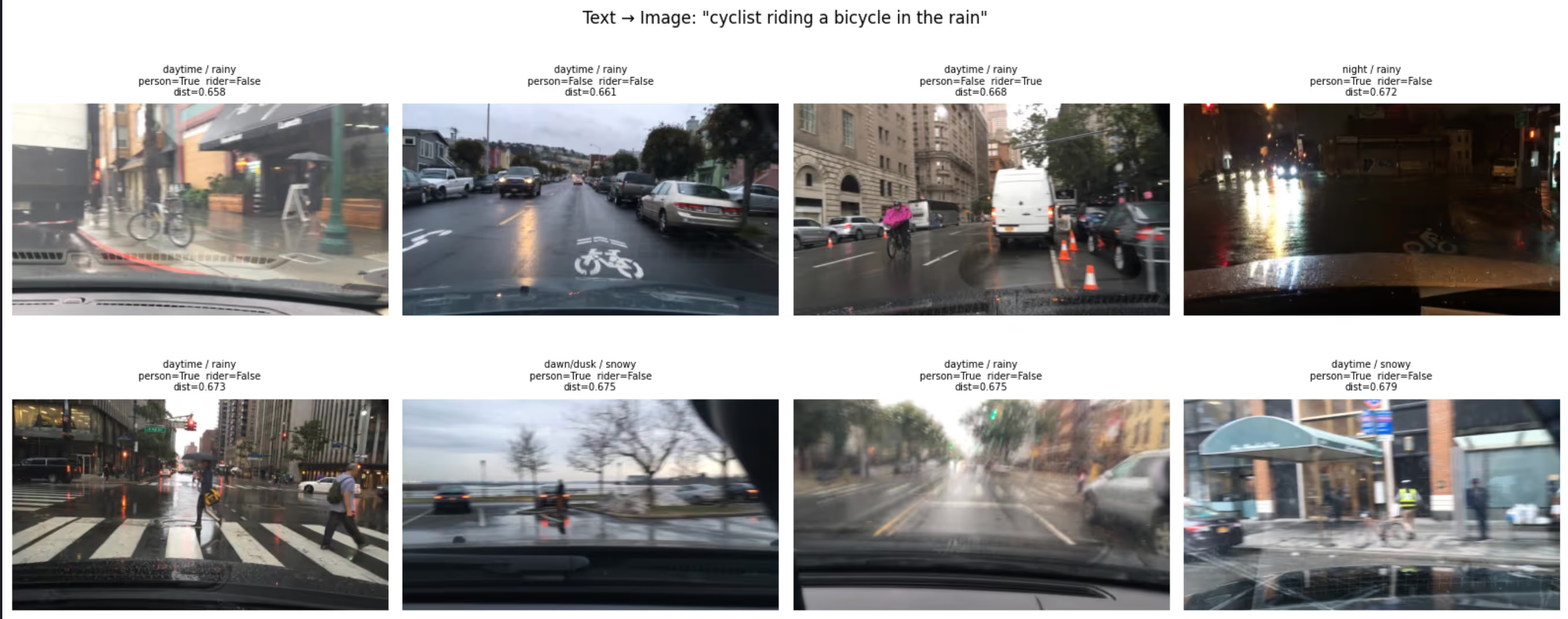
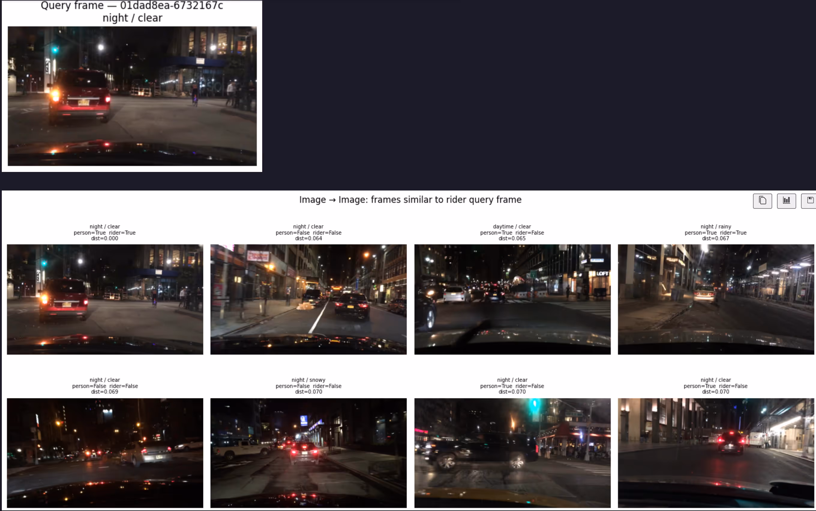
Image → Image: Pick a query frame from the rider split and retrieve visually similar frames across the full table. Useful for finding cross-split near-duplicates or unlabeled frames from the same road segment.
Vector + SQL pre-filter: The same query with and without a SQL pre-filter shows the difference clearly. "Pedestrian crossing at an intersection" returns a mix of daytime and nighttime frames without a filter. Adding timeofday = 'night' restricts vector scoring to nighttime frames only. Neither SQL alone (no visual signal) nor CLIP alone (no metadata constraint) can do this.
tbl.search(vec, vector_column_name="clip_embedding")
	.where("timeofday = 'night'", prefilter=True)
	.metric("cosine").limit(8).to_pandas()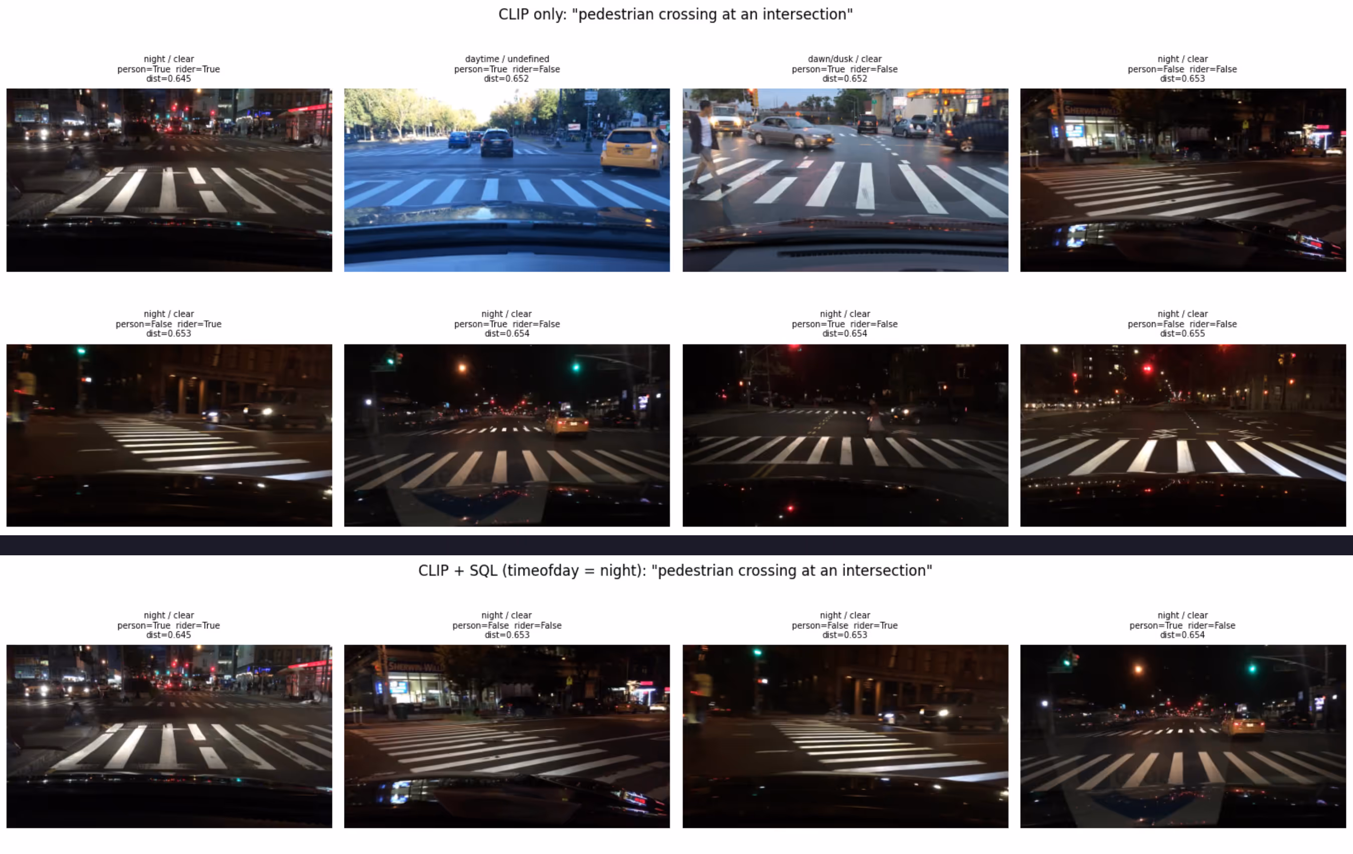
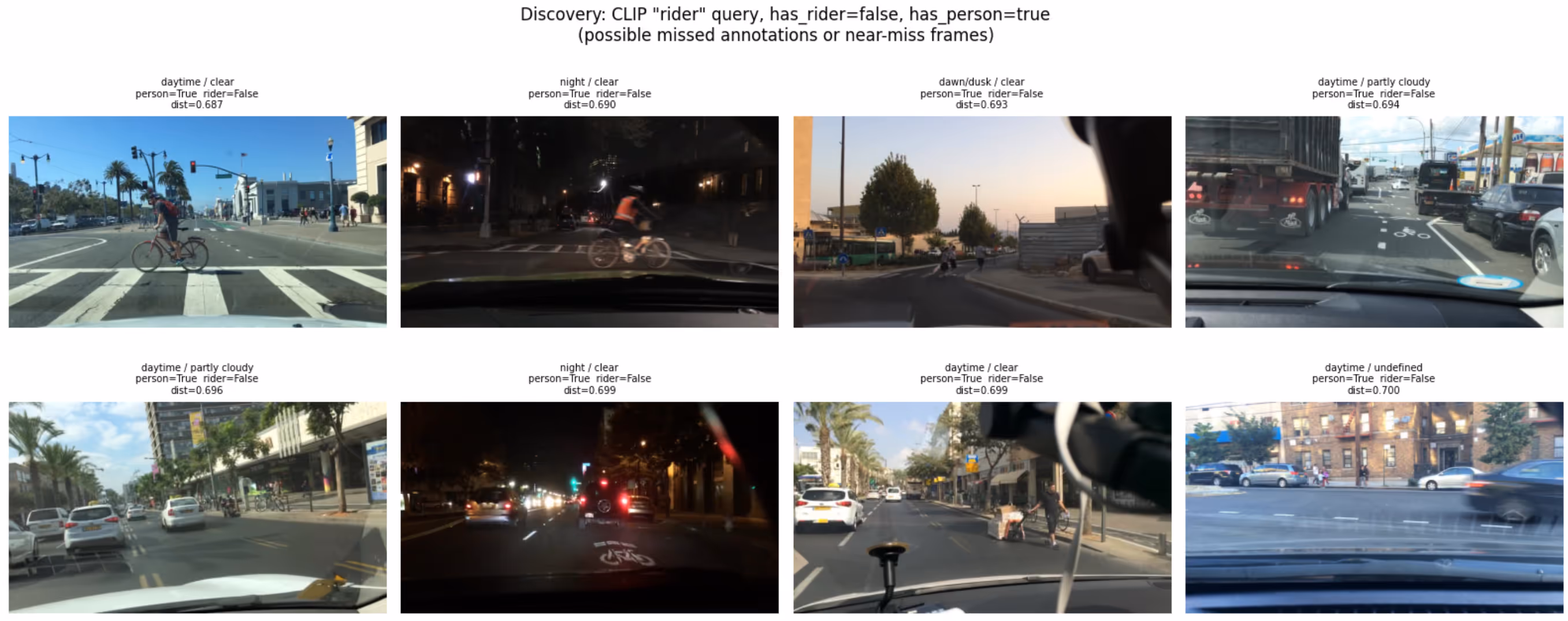
Discovery (unannotated edge cases): You can find frames that CLIP scores as "rider-like" but have has_rider = false. These are candidates for missed annotations or genuine near-miss frames, exactly the kind of finding that's impossible to reach with SQL alone.
vec = encode_text("person riding a bicycle or motorcycle on the road")

tbl.search(vec, vector_column_name="clip_embedding")
	.where("has_rider = false AND has_person = true", prefilter=True)
	.metric("cosine")
  	.limit(8)
  	.to_pandas()
SQL, FTS, and vector search are not three different systems here. They're three different index types on different columns of the same Lance table, combined in a single WHERE clause.
Materialized Views
Training Splits That Refresh Themselves
With Materialized views, you define a transformation once and materialize it as a versioned table. When new data arrives, only the affected rows are processed.
A training split is a materialized view: a named LanceDB table defined by a some filtered view, commonly via a SQL clause. Creating one from a table is just 2 lines:
conn = geneva.connect("data/bdd100k/lancedb")
tbl  = conn.open_table("bdd100k")

query = tbl.search().where("has_rider = true AND split = 'train'")
mv    = conn.create_materialized_view("bdd100k_rider_train", query)
mv.refresh()

print(f"{mv.count_rows()} rows  (version {mv.version})") # 80,000 → 3,590 rows  (version 1)
The training script opens the view same as any other LanceDB table:
db  = lancedb.connect("data/bdd100k/lancedb")

tbl = db.open_table("bdd100k_rider_train")
When new footage is ingested and backfilled into a column, one call per view incrementally adds only the new rows. For example, here's the refresh call after adding 500 rows to parent table:
mv = conn.open_table("bdd100k_rider_train")
mv.refresh() # [bdd100k_rider_train]  3,590 → 3,705 rows  (+115)  version 2
Given a checkpoint, you can always reproduce the exact data it was trained on by reopening the table at that version. No external versioning system needed.
Training
Load data from your multimodal lakehouse to PyTorch training loops without performance loss
Creating a PyTorch DataLoader from a LanceDB DataLoader is pretty straighforward. Open the materialized view in LanceDB, create a Permutation, hand it to the PyTorch DataLoader:
from torch.utils.data import DataLoader

db = lancedb.connect("data/bdd100k/lancedb")
tbl = db.open_table("bdd100k_rider_train")
perm = (    Permutation.identity(tbl)
			.select_columns(["image_bytes", "ann_categories", "ann_bboxes"]))

loader = DataLoader(perm, batch_size=64)
💡 Both LanceDB table and the Permutation object can be used to create a PyTorch DataLoader. But using a table Permutation is more flexible as it provides built in helpers to efficiently filter, shuffle, create splits etc.
LanceDB's on-disk layout provides fast random access at row level, allows faster iteration, with simple pure random shuffling faster than traditional data streaming setups like Parquet-shards or WebDataset. This keeps GPU utilization high even on loading multimodal datasets, allowing you to achieve close to theoretical peak GPU Model Flops Utilization (MFU) of your workload.
Results
GPU runs are on the full BDD100K (80k frames), over 10 epochs using A100 GPUs with a batch size of 64 and AMP enabled. The baseline is the COCO pretrained checkpoint evaluated on each curated val view.
The improvements in recall and mAP are clear — the model catches significantly more of the objects it was previously missing. No external data was added; only the training distribution was corrected by curating the right slices from the existing dataset.
What happens when new data arrives?
The sequence below indicates what happens when hundreds of hours of new frames arrive the following week:
- Ingest new footage
- Backfill increments only new rows
- Refresh all views
- Rerun training against updated views
- Checkpoint logs a new table version
No manifest regeneration, pipeline rewrite, or team handoff. The view names don't change, the training command doesn't change. Only the version number increments, and the new checkpoint is linked to the new dataset/table version.
Code
The full implementation is in this repository. The README file has step-by-step commands for each stage. The --synthetic 500 flag generates mock frames to verify the whole pipeline locally in minutes before committing to a full BDD100K download.