
At first glance, dataset curation looks like a search problem. But the search is the easy part − a simple vector search narrows down on thousands of candidates in seconds. The hard part with curation is everything that comes after: experimentation, exploration, reusability and reproducibility.
In traditional data stacks, curation is especially messy when data is multimodal, because the embeddings, raw multimodal bytes, text and metadata tend to be duplicated or spread across multiple systems. A few weeks in, the indexes may drift from the records they pointed at (because the records may have changed, or new ones landed), and the version of the data the decision was originally made against might no longer exist.
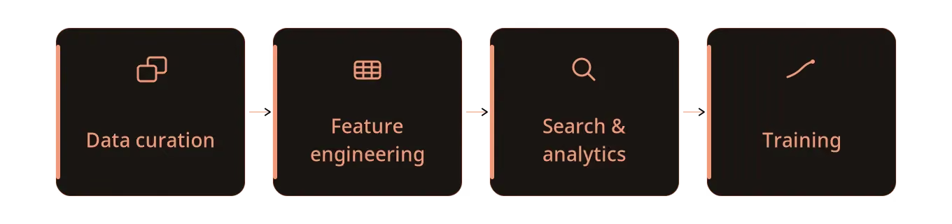
Curation is typically the first stage of an ML lifecycle that LanceDB, as a multimodal lakehouse, is built to serve end-to-end — from raw data through feature engineering, search and analytics, and training.
When we say “curation” in this post, we refer to a specific set of operations (but not limited to): filtering, search, deduplication, enrichment, sampling, inspection, materialization, and versioning of the data, so that future users of the dataset can easily inspect, debug and reproduce what was done in the past.
💡 Curation vs. Feature Engineering
The line between dataset curation and feature engineering can often get blurry, but they address different needs of the ML lifecycle.
• Curation uses the available signals to decide which subset moves forward.
• Feature engineering creates new signals: derived columns, computed scores, fresh embeddings.
The two are complementary. This post stays on the curation side; feature engineering is the subject of the next post in this series.
In the rest of this post, we’ll walk through each of the above steps, explaining how LanceDB makes it simple to manage training datasets that span images, text, video, audio, and beyond.
Curation is a universal problem
Whatever the modality (images, text, video, audio, nested fields), curation tends to surface the same handful of operations, not necessarily in the same order as the sequence below:
- Filter: Which rows can we drop on metadata alone, before reading any bytes? Poor quality records, wrong language, wrong classes.
- Search: What does the neighborhood of a particular row look like? Are there near-duplicates, edge cases, or clusters worth a second look?
- Dedupe: Are we training on the same thing twice? Is there duplication at the file level, the byte level, or the semantic level?
- Enrich: Do we need to bring outside data into the table — labels, access-permission rules, metadata, or a chunked view of the rows — before the dataset is ready downstream?
- Sample: Once a candidate pool exists, what mix do we actually want to keep: random, stratified, source-weighted, or edge-case-biased?
- Inspect: What do these rows actually look like? An image grid, a transcript snippet, a key-frame strip, an action plot.
- Materialize: How do we hand the surviving rows to the next stage as a durable artifact, and not an ad hoc notebook or throwaway script?
- Version: How will the next person on the team reproduce this exact subset six weeks from now?
A researcher curating a corpus of image-text, web-text, video, or audio will run through some version of this list whether they realize it or not. The columns they touch during the filtering/deduping stage may differ, but the questions being asked are similar.
The rest of this post walks through these curation primitives and why they matter. We’ll showcase LanceDB patterns for each operation, including the data it runs on, and the audit trail of what it produced (while all data and artifacts live in one place). This keeps curation workflows streamlined and decisions reproducible.
Filter on existing metadata
Filtering during data curation typically looks like a funnel: you chain a sequence of predicates against existing columns, record the row count after every one, and inspect a trail of numbers that show how the candidate set ID reduced to the relevant, task-specific subset required downstream.
For an image-text corpus like LAION-1M, a reasonable first pass might keep successful records, drop anything flagged for safety, setting a minimum CLIP image–text similarity score, and demanding a minimum image resolution. In LanceDB, you can specify this kind of chain as a SQL-style filter string:
import lancedb

db = lancedb.connect("hf://datasets/lance-format/laion-1m/data")
table = db.open_table("train")

filters = [
    "status = 'success'",
    "status = 'success' AND caption IS NOT NULL AND length(caption) > 0",
    "status = 'success' AND caption IS NOT NULL AND length(caption) > 0 AND NSFW = 'UNLIKELY'",
    "status = 'success' AND caption IS NOT NULL AND length(caption) > 0 AND NSFW = 'UNLIKELY' AND similarity > 0.28",
    "status = 'success' AND caption IS NOT NULL AND length(caption) > 0 AND NSFW = 'UNLIKELY' AND similarity > 0.28 AND width >= 256 AND height >= 256",
]
for f in filters:
    print(f"{table.count_rows(filter=f):>10,d}  {f.split(' AND ')[-1]}")
The results from the funnel and the row counts at each stage look something like this:
 1,162,252  status = 'success'
 1,162,246  length(caption) > 0
 1,079,113  NSFW = 'UNLIKELY'
 1,078,854  similarity > 0.28
   604,684  height >= 256
The whole funnel runs against the same Lance table that holds image assets alongside the metadata and indexes: no need to sync between a metadata DB, a feature store, and multiple other systems.
Scalar indexes speed up filter queries
The Lance-formatted version of HotpotQA, a popular information retrieval benchmark on Hugging Face, ships with bitmap indexes on the level and type columns. This means filters on those columns are effectively free, even on millions of rows:
db = lancedb.connect("hf://datasets/lance-format/hotpotqa-distractor-lance/data")
tbl = db.open_table("train")

print(tbl.count_rows())                                             # 90,447
print(tbl.count_rows(filter="level = 'hard'"))                      # 15,661
print(tbl.count_rows(filter="level = 'hard' AND type = 'bridge'"))  # 12,451
Stack predicates to avoid reading bytes
OpenVid-1M is a video dataset that carries multi-axis quality scores that don’t exist for static images: aesthetic_score, motion_score, temporal_consistency_score, and camera_motion. Stacking them in one predicate helps avoid reading unnecessary bytes downstream by dropping visually flat clips, clips that are either frozen or shaking, frame-to-frame instability, and locked-off shots in a single pass:
/
db = lancedb.connect("hf://datasets/lance-format/openvid-lance/data")
tbl = db.open_table("train")  # 937,957 clips

tbl.count_rows(filter="""
    aesthetic_score > 4.0
    AND motion_score BETWEEN 0.2 AND 0.8
    AND temporal_consistency_score > 0.7
    AND camera_motion != 'static'
""")
Using these techniques, it’s possible to rapidly narrow down on relevant subsets of the data during EDA, no matter the modality, even on a dataset that’s potentially petabytes in size.
Search: find similar examples and edge cases
Filters get us a smaller pool, but only when we already know what to filter on. The harder questions during curation are open-ended: what does this corner of the dataset look like, are there more examples like the one we just flagged, is there a cluster of near-duplicates worth a closer look? At very large (petabyte-) scale, this calls for semantic search or full-text search over an index.
LanceDB exposes vector, full-text, and hybrid search through a .search() builder, and the results come back alongside the same metadata and raw bytes already in the table. LAION ships with a prebuilt FTS index on caption, so a keyword scan can almost immediately find relevant results over a million-row image corpus:
hits = (
    table.search("music festival", query_type="fts")
         .select(["caption", "_score"])
         .limit(5)
         .to_polars()
)
shape: (5, 2)
┌─────────────────────────────────┬───────────┐
│ caption ┆ _score │
╞═════════════════════════════════╪═══════════╡
│ African Caribbean Food and Mus… ┆ 15.147776 │
│ North Music Festival 2020 ┆ 14.692194 │
│ Moonrunners Music Festival 5 ┆ 14.692194 │
│ Synthesis Music Festival (aka … ┆ 14.428536 │
│ Summer Music Festival Wrap Up ┆ 13.881918 │
└─────────────────────────────────┴───────────┘The same builder switches to a vector query by passing an embedding instead of a string (table.search(some_embedding, vector_column_name="img_emb")), and to hybrid queries by combining both via query_type="hybrid". From a curation perspective, this means we can pivot between text-based search (“find me captions that mention X”) and multimodal search (“find me images that look like Y”) without needing to retrieve from two different systems that expose different APIs.
Dedupe: catching obvious duplicates
Duplicates show up in every large multimodal corpus: the same product photo uploaded under five URLs, the same news image re-encoded by three CDNs, or the same robot trajectory landing in two episode segments. Training on duplicates inflates the loss surface for whatever’s overrepresented and silently biases the model.
A cheap first cut during curation is to compute a perceptual hash (pHash) for each candidate image and group rows whose hashes match. The following snippet shows how to run that on a 2,000-row sample of filtered LAION rows:
import io
from collections import defaultdict

import imagehash
from PIL import Image

# Pull a sample of clean candidates from the LAION table
sample = (
    table.search()
         .where("status = 'success' AND NSFW = 'UNLIKELY' AND similarity > 0.3 AND width >= 256")
         .select(["caption", "url", "image"])
         .limit(2000)
         .to_arrow()
)

# Compute pHash for each image and group identical hashes
hash_to_rows = defaultdict(list)
for i in range(sample.num_rows):
    img = Image.open(io.BytesIO(sample["image"][i].as_py()))
    hash_to_rows[str(imagehash.phash(img))].append(i)

clusters = {h: rs for h, rs in hash_to_rows.items() if len(rs) >= 2}
print(f"Sample rows:                {sample.num_rows}")
print(f"Unique pHashes:             {len(hash_to_rows)}")
print(f"Clusters with >= 2 rows:    {len(clusters)}")
print(f"Rows in duplicate clusters: {sum(len(rs) for rs in clusters.values())}")
Sample rows: 2000
Unique pHashes: 1753
Clusters with >= 2 rows: 245
Rows in duplicate clusters: 492Roughly a quarter of the cleaned LAION-1M sample lands in a pHash cluster, mostly pairs and triples that look like the same product photo or stock image reposted across URLs. Note that pHash doesn’t need to be written back to the Lance table here: it could stay a curation-time helper that informs which rows to drop or merge, or it could be materialized to a new column to be reused later (which is essentially like computing a new feature).
pHash works on pixel-level patterns, so it catches obvious re-encoded/resized images cheaply but misses duplicates that have been cropped, rotated, or recolored. Real-world pipelines typically address this gap with a two-layer approach: other hash variants (dHash, wavelet hash) tuned to different transforms, and content-based dedupe using image embeddings from CLIP or DINOv2, which match images by what they show rather than how their pixels look. Webster et al. ( On the De-duplication of LAION-2B, 2023 ) used CLIP-feature nearest-neighbor matching to estimate that roughly 700M images, about 30% of LAION-2B, are duplicates, most of which never show up in a pHash pass.
Enrich and assemble
Curation often involves bringing more data into the candidate pool, not just narrowing it down: joining in safety labels, attaching the access rules that control which users or groups can see each row, or chunking documents into per-passage rows before the dataset is ready downstream.
As a columnar lakehouse format, Lance is optimized for search, native indexing, and cheap data evolution on multimodal data. As such, joins are not a storage-format primitive. When enriching an existing Lance table with data from external sources, the typical pattern is to perform joins upstream using a compute engine such as DuckDB, Spark, Polars or DataFusion, and then materialize the joined/enriched result into a LanceDB table. The example below shows this pattern with DuckDB, though similar join queries apply in other systems too.
import duckdb
import lancedb

db = lancedb.connect("./lancedb")
tbl = db.open_table("docs")

# Do the joins in DuckDB or any other compute engine
# Emit one row per serving entity (a chunk)
joined = duckdb.sql("""
    SELECT d.tenant_id, d.doc_id, d.chunk_id, d.text, d.vector,
           m.source_uri, perm.allowed_group_ids, c.customer_tier
    FROM docs_source d
    LEFT JOIN metadata_source    m    ON d.doc_id    = m.doc_id
    LEFT JOIN permissions_source perm ON d.doc_id    = perm.doc_id
    LEFT JOIN customer_source    c    ON d.tenant_id = c.tenant_id
""").arrow()

# Upsert the materialized result into LanceDB by its logical key
(
    tbl.merge_insert(["tenant_id", "doc_id", "chunk_id"])
       .when_matched_update_all()
       .when_not_matched_insert_all()
       .execute(joined)
)
merge_insert is LanceDB’s join-on-key upsert method: matched rows update in place, while unmatched rows perform insert. It allows incremental refreshes, backfills, and materialized-table maintenance on a single machine. Note that it’s not a replacement for a relational join engine, but it is a useful tool to curate and prepare data for downstream tasks during initial data exploration.
Sample: shape the train/test distribution
Once the right data is assembled and deduplicated, the data is sampled to prepare train/test splits. A common pattern for this is stratified sampling: bin the candidate pool on an attribute we want preserved (CLIP similarity, resolution, language, source, etc.), then split inside each bin. Train and test share similar overall distributions, but the rows stay disjoint.
Lance tables are Arrow-native, so any compute engine that speaks Arrow can read them zero-copy and run its own primitives directly on the rows. Polars has the building blocks for stratification (qcut for quantile binning, over() for grouped windowed operations), which compose into a 95/5 stratified split of LAION candidates by CLIP-similarity quintile in a few lines:
import polars as pl

clean_filter = (
    "status = 'success' "
    "AND caption IS NOT NULL AND length(caption) > 0 "
    "AND NSFW = 'UNLIKELY' "
    "AND similarity > 0.28 "
    "AND width >= 256 AND height >= 256"
)

# Lance pushes the filter into the scan, so only the surviving rows
# come back as a polars dataframe.
candidates = (
    table.search()
         .where(clean_filter)
         .select(["key", "caption", "similarity", "width", "height"])
         .to_polars()
)

# Bin similarity into 5 quantiles and stratify the 95/5 split
candidates = candidates.with_columns(
    pl.col("similarity").qcut(5, labels=["q1", "q2", "q3", "q4", "q5"]).alias("sim_bin")
)
shuffled = pl.int_range(pl.len()).shuffle(seed=42).over("sim_bin")
cutoff   = (pl.len() * 0.95).cast(pl.Int64).over("sim_bin")
splits   = candidates.with_columns((shuffled < cutoff).alias("is_train"))

print(splits.group_by("is_train").agg(
    pl.len().alias("rows"),
    pl.col("similarity").mean().round(4).alias("mean_sim"),
    pl.col("similarity").std().round(4).alias("std_sim"),
).sort("is_train"))
shape: (2, 4)
┌──────────┬──────┬──────────┬─────────┐
│ is_train ┆ rows ┆ mean_sim ┆ std_sim │
╞══════════╪══════╪══════════╪═════════╡
│ false ┆ 25 ┆ 0.3318 ┆ 0.0255 │
│ true ┆ 475 ┆ 0.3318 ┆ 0.029 │
└──────────┴──────┴──────────┴─────────┘The output above shows that the train and test have the same mean similarity (0.3318) and near-identical standard deviations: we’ve obtained the same distribution shape with disjoint rows, which is exactly what we may want for training.
Being built on an Arrow-native foundation lets Lance tables interoperate with many of the same tools that researchers already use in their workflows: Polars, DuckDB, or Pandas.
Inspect: keep a human in the loop
Before persisting the curated subset to disk, it’s worth it for a human to visually inspect some of the samples and ask whether the dataset matches their desired mental model. Lance reads only the columns you asked for, so pulling 16 captions plus JPEG bytes from a million-row table is a small, targeted scan:
import io
from PIL import Image

sample = (
    table.search()
         .where("similarity > 0.32 AND width >= 256 AND height >= 256 AND NSFW = 'UNLIKELY'")
         .select(["caption", "image"])
         .limit(16)
         .to_arrow()
)

n = sample.num_rows
images   = [Image.open(io.BytesIO(sample["image"][i].as_py())) for i in range(n)]
captions = [sample["caption"][i].as_py()                       for i in range(n)]
# render however you like: image grid in Jupyter/Marimo notebook, save to disk, etc.
A quick visual pass by a human can catch what metrics like counts or hashes can’t: low-signal frames or captions that don’t make sense. When caught at the curation stage, it costs an added minute or two; but when caught after the model is trained, they cost the entire duration of that run, in addition to human time.
Materialize the curated subset
To hand the work off to a downstream stage (feature engineering, labeling, training), the surviving rows need to become a durable artifact: a new Lance table (with a new version tag) the next workflow can open directly.
One of the biggest benefits of Lance is that the JPEG bytes, captions, embeddings, and metadata all live in the same table, so writing the curated subset is a single call and reading any row downstream is a single fetch. The filtered scan can be streamed as a RecordBatchReader via .to_batches(), which keeps the write tractable on tables with hundreds of millions of rows:
import lancedb

local_db = lancedb.connect("./curation_outputs")

clean = local_db.create_table(
    "laion_clean_candidates",
    data=table.search().where(clean_filter).to_batches(),
    mode="overwrite",
)
print(f"Rows:     {clean.count_rows():,}")
print(f"Versions: {[v['version'] for v in clean.list_versions()]}")
Rows: 604,684
Versions: [1]What is stored at ./curation_outputs/laion_clean_candidates.lance is a self-contained Lance table: every surviving row carries the desired image bytes, caption, similarity score, CLIP embedding, and full provenance from the source, with an independent version history starting at 1. The next user of the dataset can open it and read whatever they need without needing to write ad hoc scripts that coordinate between multiple systems.
Version decisions, not just data
Curation is an inherently iterative process. New records arrive. Old ones change. A human reviewer flags a class of duplicates that pHash missed, and we need to drop them in a second pass. Every time an evaluation surfaces a regression, or the dataset changes, the candidate set must also change. At the same time, we may still want the previous version back when the time comes to debug or review decisions.
Lance versions every data mutation automatically: each write creates a new version of the dataset, and older ones stay on disk (until a cleanup job is run). The version stamp ([1]) is the first entry in a growing history we can tag, check out, and diff against. The output below is from a small materialized slice (the same operations work unchanged on the full-scale dataset).
# Tag the materialized baseline so we can re-open this exact version later
clean.tags.create("clean-v1-2026-05-21", clean.version)

# A few weeks later: an eval shows the similarity threshold was too loose;
# tighten it from 0.28 to 0.32 by dropping the bottom of the candidate set.
clean.delete("similarity < 0.32")
print(f"After tightening: version={clean.version}, rows={clean.count_rows():,}")

# The original baseline is still on disk, addressable by tag
baseline = local_db.open_table("laion_clean_candidates")
baseline.checkout("clean-v1-2026-05-21")
print(f"Baseline:         version={baseline.version}, rows={baseline.count_rows():,}")
After tightening: version=2, rows=1,190
Baseline: version=1, rows=2,000At a future date, a training run that pinned clean-v1 still reads exactly the dataset it was evaluated against. A second run that uses v2 captures a different decision, with the diff between the two versions sitting in the same Lance table. As a researcher, this simplifies the workflow to reproduce any given result.
What this unlocks next
Curation is done at the earlier stages of the ML lifecycle. The bulk of the curation steps shown above ran against the same Lance table on a single machine (in many cases, directly scanning/filtering data from the Hugging Face Hub), without needing to manage data across multiple systems to paint the full picture.
LanceDB keeps blobs, text, embeddings, metadata, and indexes in one versioned table so curation runs against exactly the rows and indexes pinned to that version. Any future subset can be pinned to a new version that downstream stages may reference unambiguously.
All datasets shown in this post can be found on the Hugging Face Hub in Lance format, queried directly by pointing to their respectivehf:// URIs. See the documentation for a list of available datasets that are similar to your use case. If you create a Lance dataset of your own, uploading it to the Hub makes it immediately explorable, filterable, and searchable for anyone with LanceDB installed. Our guide on uploading Lance datasets to the Hub walks through every step end-to-end.
The curated dataset we ended up with is the input to everything that comes after: feature engineering (computing new signals as derived columns), search and analytics (running production retrieval against the curated rows), and training (sampling batches from the same Lance dataset that captured every curation decision). The LanceDB Multimodal Lakehouse is purpose-built for these kinds of end-to-end training data preparation workflows, so look out for more upcoming posts that walk through the other stages.
Browse some existing Lance datasets on the Hugging Face Hub, create and curate your own, and spread the word! 🚀