Make Handwritten Notes Searchable: Optimizing an OCR Pipeline with LanceDB

As anyone who’s been to the doctor can attest, handwritten prescriptions are no mean feat to read. Building an OCR pipeline for this kind of handwriting is harder than it looks because scanned notes can be messy, fuzzy, and hard to discern for both humans and agents.

To do question-answering on a handwritten note, it’s tempting to build a retrieval system around a vision-language model that reads the images directly. The system retrieves a set of candidate images for a query, hands them to the model, and lets it reason over the pixels to answer the question. However, the problem with this is twofold:

• VLMs may work reasonably well over a few samples, but problems show up at scale. Once the corpus grows to millions of documents and queries start arriving in volume, every search turns into one or more multimodal inference calls, latency climbs, and the token bill grows with it.
• Reasoning over pixels can be lossy and inadequate. The model (which may not be domain-aware) re-reads the same fuzzy prescription every time it resurfaces as a candidate, and fuzzy inputs invite inconsistent or hallucinated answers.

There’s a cleaner and lower-cost shape for this kind of task. We could store the original images, run OCR (optical character recognition) to turn the pixels of handwriting into text, and then embed and index that text so search runs over cheap text features. The image pixels are still always available if needed: they just stop being on the hot query path, and become the evidence we fetch back when a human or agent needs to verify an answer.

In this post, we’ll build an OCR-based retrieval workflow end-to-end with LanceDB. We’ll start with a local open-source workflow, then show how the same pattern can move to LanceDB Enterprise when scale, governance, and operational execution become more important.

The two tiers: storage and retrieval

During OCR, we use a model to read each image a single time, up front, and capture the text it contains as a text feature for our storage layer. From then on, every query runs against cheap text features, and the original image is there to fetch back only when someone needs to confirm an answer.

This splits the system into two layers (storage and retrieval) that both live in LanceDB:

Storage runs upfront, once per document. Handwritten PNGs go into a LanceDB table as raw image bytes, and each enrichment step reads from that table and writes back to it. An OCR program turns the image into ocr_text, an extraction step distills that text into normalized fields and a searchable_summary, and an embedding step turns the summary into a vector. Each of those outputs becomes a column on the same row, right next to the image it came from.

Retrieval runs on demand, for every query, and it only optionally touches a VLM (the default retrieval mode is text-only). We embed the user’s question, match it with dense vector search to pull the top candidates, and optionally rerank them with a late-interaction model for token-level precision. The candidate rows carry their original image and labels along with them, so the evidence is a single lookup away when we want to inspect it in more depth.

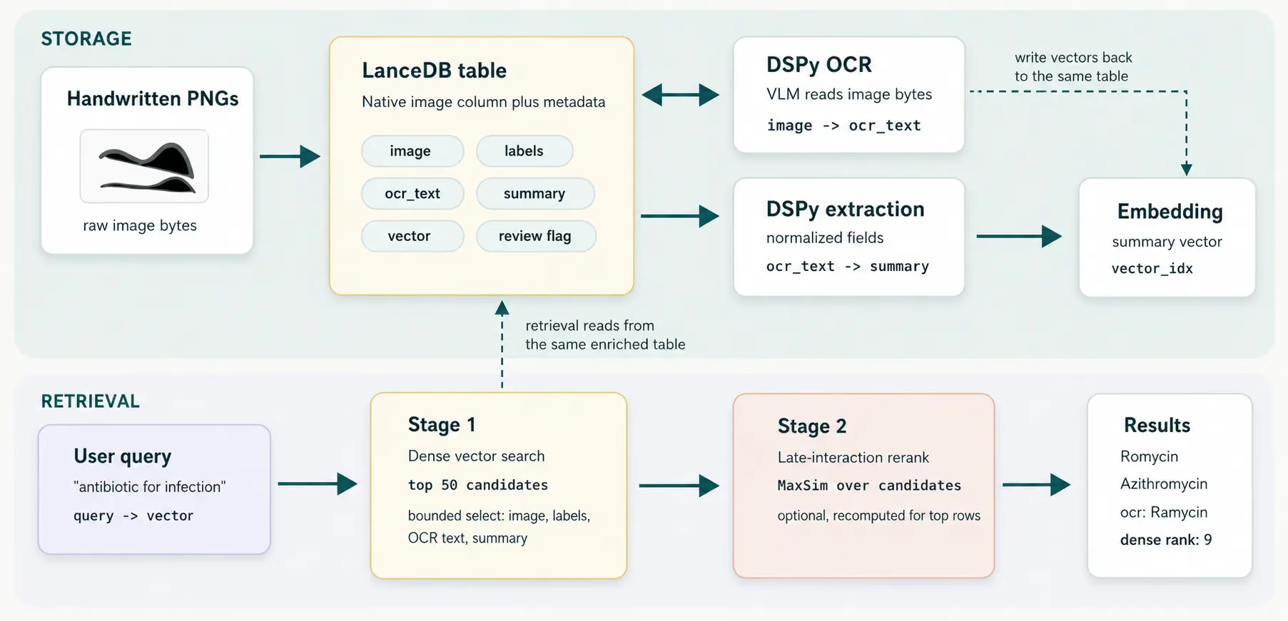
Storage runs upfront, once per document. Handwritten PNGs go into a LanceDB table as raw image bytes, and each enrichment step reads from that table and writes back to it. An OCR program turns the image into ocr_text, an extraction step distills that text into normalized fields and a searchable_summary, and an embedding step turns the summary into a vector. Each of those outputs becomes a column on the same row, right next to the image it came from.

Retrieval runs on demand, for every query, and it only optionally touches a VLM (the default retrieval mode is text-only). We embed the user’s question, match it with dense vector search to pull the top candidates, and optionally rerank them with a late-interaction model for token-level precision. The candidate rows carry their original image and labels along with them, so the evidence is a single lookup away when we want to inspect it in more depth.

Ingestion: store image bytes alongside metadata

We’ll use the Lance-formatted version of the Doctor’s Handwritten Prescription BD dataset, available on Hugging Face Hub, which you can browse or download directly. It contains 4,680 cropped PNG images of handwritten medicine names, with source-preserved train, validation, and test splits.

The original source dataset is available here on Kaggle. In this post, the test split has 780 scanned images of prescriptions and is used initially to establish the baseline, while the training and validation splits are used later during prompt optimization.

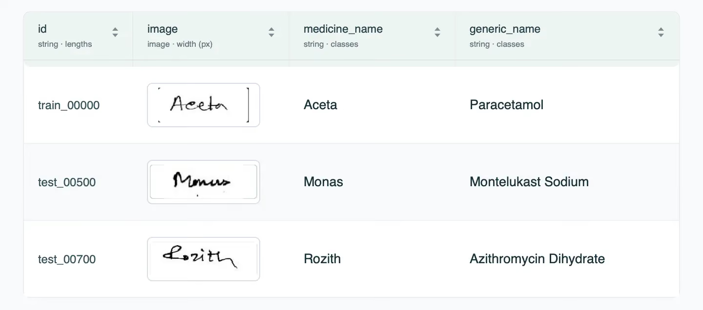
Each image is labeled with the medicine name written on it and its generic equivalent. The annotated labels are what let us evaluate OCR quality later, so we store them in the table right beside the image they describe.

Everything produced by the pipeline will live in a single LanceDB table, defined via this Pydantic schema:

from lancedb.pydantic import LanceModel, Vector

class DoctorHandwriting(LanceModel):
    # Source
    id: str
    split: str = "Testing"
    image_filename: str
    image: bytes
    # Validation labels
    medicine_name: str
    generic_name: str
    # Structured extraction
    normalized_text: str | None = None
    category: str | None = None
    is_medical: bool | None = None
    needs_human_review: bool | None = None
    searchable_summary: str | None = None
    source_dataset: str = SOURCE_DATASET
    # Retrieval
    vector: Vector(VECTOR_DIM) | None = None

The base table starts with the source image bytes, validation labels, and downstream retrieval fields. OCR gets added later as a feature column, because that’s the workflow we want to model: start with a source dataset, run a transformation, and write the result back beside the source row.

The table grows wider (i.e., more columns can be added as new features) over time, and because Lance is designed for data evolution, any backfills that add values only write new data files, leaving existing data files untouched.

The ingestion stage involves reading the “Testing” split’s ground-truth labels, ingesting each image as raw bytes, and constructing one row for each image of handwritten text:

labels = load_testing_labels()
rows = []

for i, row in enumerate(labels.iter_rows(named=True)):
    # Read the raw image bytes to ingest into LanceDB
    with open(row["image_path"], "rb") as image_file:
        image_bytes = image_file.read()
    rows.append({
        "id": f"test_{i:05d}",
        "split": "Testing",
        "image_filename": row["IMAGE"],
        "image": image_bytes,
        "medicine_name": row["MEDICINE_NAME"],
        "generic_name": row["GENERIC_NAME"],
        "source_dataset": SOURCE_DATASET,
    })

table = create_table(mode="overwrite")
table.add(rows)
table.optimize()

Here’s what the table looks like right after this stage: the handwritten scans live natively in the image column next to their labels, while later feature columns like ocr_text, searchable_summary, and vector are still waiting to be added or backfilled.

Baseline OCR pipeline

Once the images are in the table, they’re still just pixels. The useful feature we need to make this cheaper is text. By running an OCR pass over the image, its transcription can be written back to a new column, so that every image now has text features associated with it. LanceDB OSS is a great way to quickly get started because it runs as an embedded retrieval library on your local machine.

To begin, we use Google’s gemini-3.1-flash-lite as the OCR model. It’s cheap and fast enough for rapid iteration, while still strong enough to provide a decent baseline. This allows us to quickly run experiments over the full Testing split of 780 samples to gauge baseline performance.

We wrap the model call with DSPy, a modular, declarative framework for writing language model workflows as small programs rather than one-off prompts. In DSPy, a Signature defines the task contract: what inputs the model receives, what fields it should return, and the short natural-language instruction that connects the two.

The baseline signature starts with a short instruction that only asks for the handwritten medicine name:

import dspy

class HandwritingOCR(dspy.Signature):
    """Transcribe the handwritten medicine name shown in the image, exactly as written."""

    image: dspy.Image = dspy.InputField(desc="A handwritten medicine name")
    ocr_text: str = dspy.OutputField(desc="The transcribed text, exactly as written")

When using DSPy, we don’t begin with long, elaborate, hand-crafted instructions in the prompt because we want to establish the model’s default behavior first. The signature abstraction is powerful because it lets us declaratively express the desired input/output types, along with a user instruction (what we’d normally call a “prompt”). If the initial instruction is already heavily hand-engineered, it’s harder to tell what the optimizer is improving later.

In general, it’s best to let a “good prompt” be discovered by the optimizer (which improves prompts over a tangible metric), rather than spending a lot of time manually tuning it by hand (which is subjective and error-prone). Let the model write the prompts, and let the optimizer validate what works.We’ll optimize the prompts in the next section, but first, we need to establish the baseline OCR pipeline.

We first read the id, image, and medicine_name column values from LanceDB, decode the image bytes, call the DSPy reader, and write the model outputs back to the same table:

# Fetch the source image bytes and ground-truth label together from LanceDB.
image = Image.open(io.BytesIO(row["image"]))
image.load()

# Call the DSPy OCR program with the decoded image.
pred = await reader.aforward(image=dspy.Image(image))
ocr_text = pred.ocr_text.strip()

# Write OCR output back to LanceDB.
row_update = {
    "id": row["id"],
    "ocr_text": ocr_text,
    "ocr_model": VISION_MODEL,
}
row_update.update(ocr_scores(ocr_text, row["medicine_name"]))
merge_update([row_update])

Unlike traditional workflows where there are multiple sidecar files/systems, in LanceDB, everything can be written as columns in the same table. Every image record is a row in that table, and its features and metadata are columns.

The baseline OCR loop is run to generate the initial results after evaluation:

uv run python src/02_ocr.py --split Testing --overwrite
uv run python src/07_evaluate.py \
  --split Testing \
  --run-name "Gemini baseline" \
  --output outputs/baseline_results.md

Because the ground-truth labels live in the table too, evaluation is just another table read. We compare ocr_text with medicine_name (which is the ground truth), both exactly and after normalization. The table below shows the results on the test split of 780 samples. The normalized match rate is the percentage of exact matches after lowercasing and stripping out special characters. Edit distance is computed as the number of single-character inserts, deletes or substitutions needed for an exact match, measured as the Levenshtein distance.

The baseline results show that the OCR task isn’t as simple as it might seem. A normalized match rate of 54.1% means the model is reading a lot of words correctly, and a median edit distance of 0.00 tells us at least half the rows are exact after normalization. The average edit distance of 1.01 is the more interesting signal: many failures are close misses that are off by a single characeter.

Prompt Optimization: DSPy + GEPA

Once we have a baseline, the obvious temptation is to jump to a bigger, more expensive model. That may help, but we can ask a narrower question first: can the same low-cost model do better if we give it better task instructions?

This is where GEPA comes in. DSPy gives us clean abstractions (signatures and modules) to define the OCR task: image in, transcribed text out. GEPA is a genetic Pareto optimizer that then treats the instruction inside that task as something it can search over. It runs the student model on labeled examples, looks at the mistakes, asks a stronger reflection model to propose better instructions, and keeps the candidates that score well on validation examples.

For prompt optimization, the student model stays the same: gemini-3.1-flash-lite. The reflection model is stronger and more capable: gemini-3.1-pro-preview, and is used purely to suggest how to generate improved instructions by providing feedback to the student model.

Before running optimization, it’s important to define the metric we actually care about. For this task, normalized exact match matters much more than edit distance － edit distance helps distinguish “almost right” from “very wrong,” but it shouldn’t dominate the objective, so it’s down-weighted heavily compared to the normalized exact match in the objective.

# How the GEPA scoring metric looks like in practice
def score_ocr(predicted: str | None, gold: str) -> float:
    predicted_norm = normalize_text(predicted)
    gold_norm = normalize_text(gold)

    normalized_match = predicted_norm == gold_norm
    edit_sim = 1.0 - edit_distance(predicted, gold) / max(len(gold_norm), 1)

    return 0.90 * float(normalized_match) + 0.10 * max(0.0, edit_sim)

We also add a light output-shape penalty function. This doesn’t try to judge handwriting quality directly. It catches failure modes from OCR that are obviously bad for this task: returning dosage amounts, adding extra tokens, emitting special or unsupported characters, or inserting/dropping too many characters. The penalty is intentionally mild (kept at most 90% of the actual value) because the main signal should still come from the normalized match.

def output_shape_penalty(predicted: str, gold: str) -> float:
    penalty = 1.0
    predicted_norm = normalize_text(predicted)
    gold_norm = normalize_text(gold)

    # Terms that should be penalized in the output
    banned_terms = {"tab", "tablet", "cap", "capsule", "mg", "ml", "syrup", "injection"}

    if any(term in predicted.lower().split() for term in banned_terms):
        penalty *= 0.90

    if len(predicted.split()) > max(len(gold.split()), 1):
        penalty *= 0.95

    if set(predicted) & set(",/;:()[]{}"):
        penalty *= 0.95

    if abs(len(predicted_norm) - len(gold_norm)) >= 3:
        penalty *= 0.97

    return penalty

The custom metric is plugged into the dspy.GEPA module, with the required settings. Note that in this step,we need to provide the training and validation samples (that are distinct from the held-out test set).

def metric(example, pred, trace=None) -> float:
    score, *_ = score_prediction(
        predicted=pred.ocr_text,
        gold=example.ocr_text,
        metric_style="normalized_weighted_edit",
    )
    penalty, _ = output_shape_penalty(pred.ocr_text, example.ocr_text)
    return score * penalty


optimizer = dspy.GEPA(
    metric=metric,
    auto="medium",
    reflection_lm=reflection_lm,
    reflection_minibatch_size=8,
    num_threads=4,
)

optimized_reader = optimizer.compile(
    student=reader,
    trainset=trainset,
    valset=valset,
)

The optimization script is run as follows, using the “medium” setting in GEPA (that controls the number of rollouts):

uv run python src/08_optimize_ocr.py --auto medium

The run takes ~15 minutes on a laptop and uses the Gemini API for LLM calls. It reads the Training and Validation rows from the same LanceDB table as the images, and then writes the optimized DSPy program once it finishes. The Testing split is held out of the optimization loop and only comes back when we evaluate the final optimized prompt.

We found a few things worth noting for this run that really impacted the quality of results:

• The right scoring metric is crucial to the outcome. For this OCR task, normalized exact match is the most important outcome. Edit distance is useful, but it’s a secondary signal. If edit distance dominates the score, GEPA can learn prompts that produce closer wrong answers without improving exact OCR accuracy. The current metric makes normalized exact match dominate, with a small edit-distance component to help GEPA distinguish between bad and almost-right outputs.
• Randomize and subset the data. The validation set can’t just be “the first N rows,” and it doesn’t need to be huge. GEPA evaluates prompt candidates against validation examples many times, so a very large valset can spend too much of the budget on scoring and not enough on exploring alternatives. In the script, only 192-256 validation rows (out of 780) are loaded, shuffled with a seed, and then used during optimization.
• Treat optimizer settings as experimental settings. The knobs are exposed as --metric-style, --train-limit, --val-limit, and --seed because these choices affect the prompt GEPA discovers.

The optimized prompt significantly improves the held-out Testing result:

We observe a decent lift from the baseline: normalized match moves from 54.1% to 59.4%, and average edit distance drops from 1.01 to 0.87.

The optimized prompt, discovered by GEPA via a reflection language model’s feedback, looks like this:

You are an expert handwriting transcription assistant specializing in medical contexts.
Your task is to carefully read and transcribe the handwritten medicine name from the
provided image exactly as it is written.

Please follow these strict guidelines:

1. **Detailed Visual Analysis & Trailing Letters**: Analyze the handwriting stroke by stroke,
letter by letter. Pay special attention to the very end of the word: look closely for trailing
loops (e.g., a final 'e') and distinct ascenders (e.g., distinguishing a final 'd' from an 'l').
These terminal characters are crucial and must not be dropped or misread.

2. **First-Letter Capitalization & Exact Casing**: Preserve the exact capitalization seen in the
image. Carefully evaluate the relative size and stroke shape of the very first letter. If it is
noticeably larger than the subsequent letters or drawn in a distinct capital shape, output it as
an uppercase letter (e.g., output "Ketocon" or "Montex" rather than "ketocon" or "montex"). Keep
in mind that handwritten medicine names generally start with a capital letter.

3. **Domain Knowledge as a Tie-Breaker**: The primary goal is spelling accuracy. Use your
pharmacological domain knowledge of valid medicine names (e.g., recognizing "Sergel" instead of
"Zengel", "Canazole" instead of "Canazol", or "Flamyd" instead of "Flamyl") to resolve ambiguous
cursive scribbles or easily confused letters (like 'S' vs. 'Z', 'r' vs. 'n', or 'd' vs. 'l').
Lean on valid drug names when strokes are ambiguous, but never hallucinate letters that completely
contradict the clear visual evidence.

4. **Punctuation and Hyphens**: Actively look for visible punctuation, particularly hyphens (`-`),
which often separate prefixes or suffixes in drug names. Do not misinterpret a horizontal hyphen
stroke as a space, a connecting stroke, or part of a letter.

5. **Strict Whitespace Control**: Cursive text often contains uneven gaps or lifted pen strokes.
**Do not introduce spaces within a single continuous name or around hyphens.** Only insert spaces
when there is an unmistakable, deliberate physical gap indicating completely distinct words.

6. **Strict Output Format**: Provide exactly one concise transcription string. Do not include
any extra words, introductory text, explanations, punctuation outside the actual name, extra
metadata, dosage markers, or multiple guesses. Your final output must contain solely the transcribed text.

That’s quite the improvement from our naive baseline, which was simply: “Transcribe the handwritten medicine name shown in the image, exactly as written.”

The optimized prompt (none of which was written by a human at any point) contains a lot of additional guidance on what kinds of patterns to look for, to help the model perform the task better.

However, optimization isn’t magic － there’s only so much you can do with a low-cost, general-purpose model and changing things purely in prompt space. To get an even larger jump in performance, the next likely move would be a specialized OCR VLM or a fine-tuned model. LanceDB is a great fit there too, and we covered this in a previous blog post.

The useful conclusion from this section is this: before we scale our OCR pipeline to a huge dataset, we first improved it significantly from the baseline, without manually hand-engineering a prompt. The optimization run confirmed that our predictor model got better under the metrics we care about (normalized exact matches and mean edit distance). Once we’re convinced that we improved on the baseline, it then makes sense to run OCR at scale to a larger dataset.

And importantly, all the metadata, labels and raw images were stored in a single LanceDB table that manages things in one place.

Retrieval: dense search first, richer retrieval when needed

With OCR and embeddings in place, we can query our data via a retrieval system built on LanceDB. The standard search path is compact: we embed the user’s query with the same text embedder, search the vector column in LanceDB, and return the original image together with ocr_text, medicine_name, generic_name, and review metadata.

The search script wraps that path so we can run it directly:

uv run src/05_search.py "antifungal medication" --limit 3

# distance=0.1641 id=test_00597 label=Nizoder generic=Ketoconazole (Cream) ocr='Nizoder' normalized='Nizoral' category=medication review=True
# distance=0.1641 id=test_00598 label=Nizoder generic=Ketoconazole (Cream) ocr='Nizoder' normalized='Nizoral' category=medication review=True
# distance=0.2480 id=test_00177 label=Candinil generic=Fluconazole ocr='Candixil' normalized='Candixil' category=medication review=False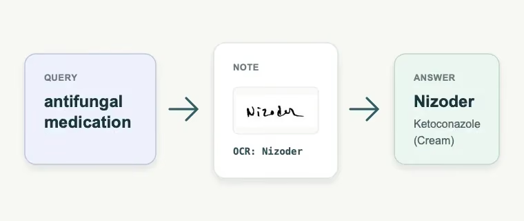

This is an important retrieval shift. We’ve converted an expensive visual reasoning problem into a cheaper text search problem. Once the handwriting becomes ocr_text and searchable_summary, a text embedding model can use what it learned during training, including that “Nizoder” and “antifungal medication” commonly occur near each other. Retrieving the nearest neighbors is then a simple, low-cost vector or hybrid search operation, and you can also benefit from full-text indexes and scalar filters that handle exact terms and review flags.

For stronger relevance, we can add a reranking pass without changing the table layout. We first ask the LanceDB dense embedding retriever for a candidate set, then apply a ColBERT-style late-interaction scorer over the candidate text’s tokens. In this example, the reranker concatenates the text from searchable_summary, ocr_text, medicine_name, and generic_name, and then scores candidates with token-level MaxSim:

uv run src/06_rerank.py "fever and body ache" --candidate-limit 10 --limit 3

# Query: fever and body ache
# Dense top results:
#   01. distance=0.6911 test_00674 Ritch (Fexofenadine Hydrochloride)
#   02. distance=0.6934 test_00202 Dancel (Ketoconazole (Shampoo))
#   03. distance=0.6955 test_00447 Lumona (Montelukast Sodium)
# Late-interaction reranked results:
#   01. late=1.7362 dense_rank=4 id=test_00367 label=Flexilax generic=Baclofen ocr='Fluxilax'
#   02. late=1.6653 dense_rank=1 id=test_00674 label=Ritch generic=Fexofenadine Hydrochloride ocr='ritcH'
#   03. late=1.5622 dense_rank=6 id=test_00097 label=Bacaid generic=Baclofen ocr='Boraid'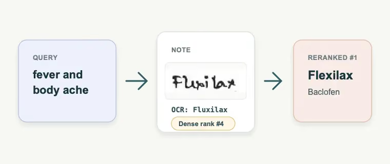

Of course, real-world queries are rarely answered by a single retrieval call like this. If we want to go further, multivector search lets a row store and search multiple vectors for one item, which is useful for late-interaction models like ColBERT or ColPali, or for separate representations of OCR text, generic names, visual tags, and page chunks. In an agentic retrieval system, it’s common to fan out into multiple concurrent searches, combine dense and exact-match evidence, rerank the strongest candidates, and return an answer built from the merged result set.

The takeaway is that we aren’t limited to using any one retrieval method in LanceDB. By adding new OCR features and keeping them alongside the indexes and rest of the data, we can layer dense search, full-text search, scalar filters, and reranking on the same table as the dataset and the downstream use cases evolve.

From fast, cheap iteration to immense scale

Once the local OCR → retrieval pipeline works well, the question changes. We have a baseline, a better OCR prompt, a retrieval path, and held-out test results. Now, the task is to run the same transformations across much larger datasets (potentially hundreds of millions of rows and beyond).

With open-source LanceDB, the OCR stage involved reading rows in hand-constructed batches, calling the DSPy reader asynchronously, and writing the ocr_text back to the table in batches. That manual approach of constructing batches works well for the fast iteration stage. It’s easy to inspect, cheap to rerun, and close to the data on disk. But in a local setup, storage and compute are tightly coupled on one machine. At production scale, we want the shape to stay the same, but the execution model needs to change. The OCR transform should become a managed table operation.

In LanceDB Enterprise, the same table storage abstraction remains, but distributed compute can run feature backfills from hundreds of millions of images on object storage. The very same OCR and extraction pipelines we validated locally can be packaged as Python UDFs, registered as computed columns, and backfilled across the table. The transformations run as distributed jobs instead of local processes, with the production environment carrying the dependencies, credentials, and runtime configuration.

Here’s what the UDF for running OCR looks like in practice:

import io

import pyarrow as pa
from geneva import udf
from PIL import Image

from dspy_programs import make_handwriting_reader

@udf(data_type=pa.string(), input_columns=["image"])
class HandwritingOCR:
    def __init__(self):
        self.reader = None

    def __call__(self, image: bytes) -> str:
        import dspy

        if self.reader is None:
            _, self.reader = make_handwriting_reader()

        pil_image = Image.open(io.BytesIO(image))
        pil_image.load()
        pred = self.reader(image=dspy.Image(pil_image))
        return pred.ocr_text.strip()

The UDF syntax lets developers express the row transform naturally. The decorator declares the output type and input column, the class keeps a DSPy reader around for reuse inside each worker, and __call__ handles one image at a time. You don’t have to write your own PyArrow batch iterator, manage row offsets, or hand-roll the merge loop.

For a production Enterprise run, the surrounding script or deployment config is where the environment is packaged: source modules, pinned dependencies, and the model API key. Once the UDF is attached to a table column, the distributed part is just the backfill call. The concurrency parameter controls the backfill parallelism for the job:

# Call the UDF in LanceDB when adding a new column
tbl.add_columns({"ocr_text": HandwritingOCR()})
result = tbl.backfill(
    "ocr_text",
    concurrency=8,
)

The computed column is added, then calling tbl.backfill schedules the work across the LanceDB Enterprise cluster in a distributed fashion, writing the computed values back to the table. As a user, you don’t need to worry about manually constructing PyArrow batches, writing multi-processing code, and handling failures.

During the initial stages, using LanceDB OSS makes sense because it allows you to move quickly, find the better prompt, and validate the retrieval flow. Eventually, scale and performance issues creep up, so it then makes sense to use LanceDB Enterprise to run the same feature engineering pattern without significant changes to the logic.

Production is about more than just scale

As the workflow scales to production-size datasets (hundreds of millions of rows and beyond), the table becomes more than just a collection of rows. It’s now the system of record for a document-intelligence workflow, containing source images, labels, OCR outputs, prompt and model versions, extraction fields, vectors, indexes, and review flags that all move and evolve independently.

For any dataset in production, the workloads evolve along with data itself. We may have more documents, higher-resolution images, new batches arriving over time, and multiple feature jobs running against the same table. New embedding models become available, so more experiments get queued up. Storage needs to grow continuously, and compute needs to scale independently so that OCR, extraction, embeddings, re-OCR experiments, and reranking features don’t all compete for resources on one giant local machine.

The operational side also gets more elaborate. Because doctors’ notes are medical-adjacent documents, access control, governance, auditability, and monitoring become integral to the workflow. Long-running backfills need to be trackable and resumable. Feature columns must carry enough context to know which model or prompt produced them. Review state should live beside the generated text it qualifies.

Human validation always stays in the loop. needs_human_review is a first-class column, and the original image bytes remain attached to every row. OCR makes retrieval cheaper and faster; it doesn’t become the source of truth. These are the main areas in which LanceDB Enterprise adds value: the same table-centered workflow, with managed scale, governance, and reliability around it.

Conclusions

The example shown above highlights why building an OCR pipeline for retrieval is far more than “store embeddings and run vector search.” LanceDB becomes the data management layer for the whole OCR improvement loop. We start with fuzzy handwritten images of doctors’ notes, turn them into searchable text, optimize our prompts, measure retrieval failures, and keep the original evidence attached the whole way.

Prompt optimization is a great lever to have at your fingertips, but handwriting OCR is a difficult task that imposes a real ceiling on how much improvement we can get out of prompts alone. The underlying model still needs a certain degree of domain-specific competence to visually decode ambiguous strokes, spacing, abbreviations, and shorthand to succeed on most counts.

Fine-tuning a reasonably competent base model can help: we’d start with a VLM that’s already good at handwritten OCR, ideally in the same domain, then fine-tune it on this dataset so it learns the handwriting and medical shorthand directly. In our earlier post on faster VLM fine-tuning with materialized model features in LanceDB, we showed how materializing expensive vision model features once can make that loop cheaper across experiments.

Combining prompt optimization with fine-tuning can yield compounding results. Fine-tuning improves the underlying model’s capability; GEPA (and other optimizers) improve the prompt/program around the model, including which fields to extract, how to preserve uncertainty, how to normalize outputs, and when to avoid guessing. Each stage can be measured with exact match, normalized exact match, edit distance, and other structured-field accuracy metrics, increasing confidence in the end-to-end retrieval pipeline.

LanceDB makes this entire loop practical, because the raw data, derived features, indexes, and experiment versions all live together. It’s straightforward to begin by running the workflow locally with LanceDB OSS, but when the workflow needs to run over much larger datasets with governance controls, LanceDB Enterprise gives it a clear path to production scale. You can reproduce the workflow shown in this post by checking out the code in the source repo, and while you’re at it, give LanceDB a star on GitHub!

‍