From Messy PDFs to Verifiable Answers with LiteParse and LanceDB

Corporate PDFs like annual ESG and sustainability reports are some of the most information-rich documents around: hundreds of pages of narrative woven together with tables, charts, and figures. Analysts and auditors comb through them for specific facts, and every number gets traced back to its source. That source is often a single page out of two hundred. To us these reports read like ordinary documents, but to a retriever they’re tangled bundles of text, tables, and figures, with the facts people want stranded at the boundaries between them.

If we flatten all of that structure too early, we lose the exact evidence the agent needs later. We also lose the ability to inspect what went wrong. Was the page parsed badly? Did chunking break up the table? Did the retriever find the right page but miss the related figure? Without a structured evidence layer, those questions are painful to answer.

Before building sophisticated agent pipelines, it’s worth thinking about how to get the evidence layer right — after all, as they say, “context is king”. PDFs should be parsed in a way that preserves the connectivity between text, page screenshots, extracted figures, metadata, embeddings, blobs, and other entities. It’s also important to store those pieces such that retrieval can combine page-level, chunk-level, and asset-level signals without losing the original page identity.

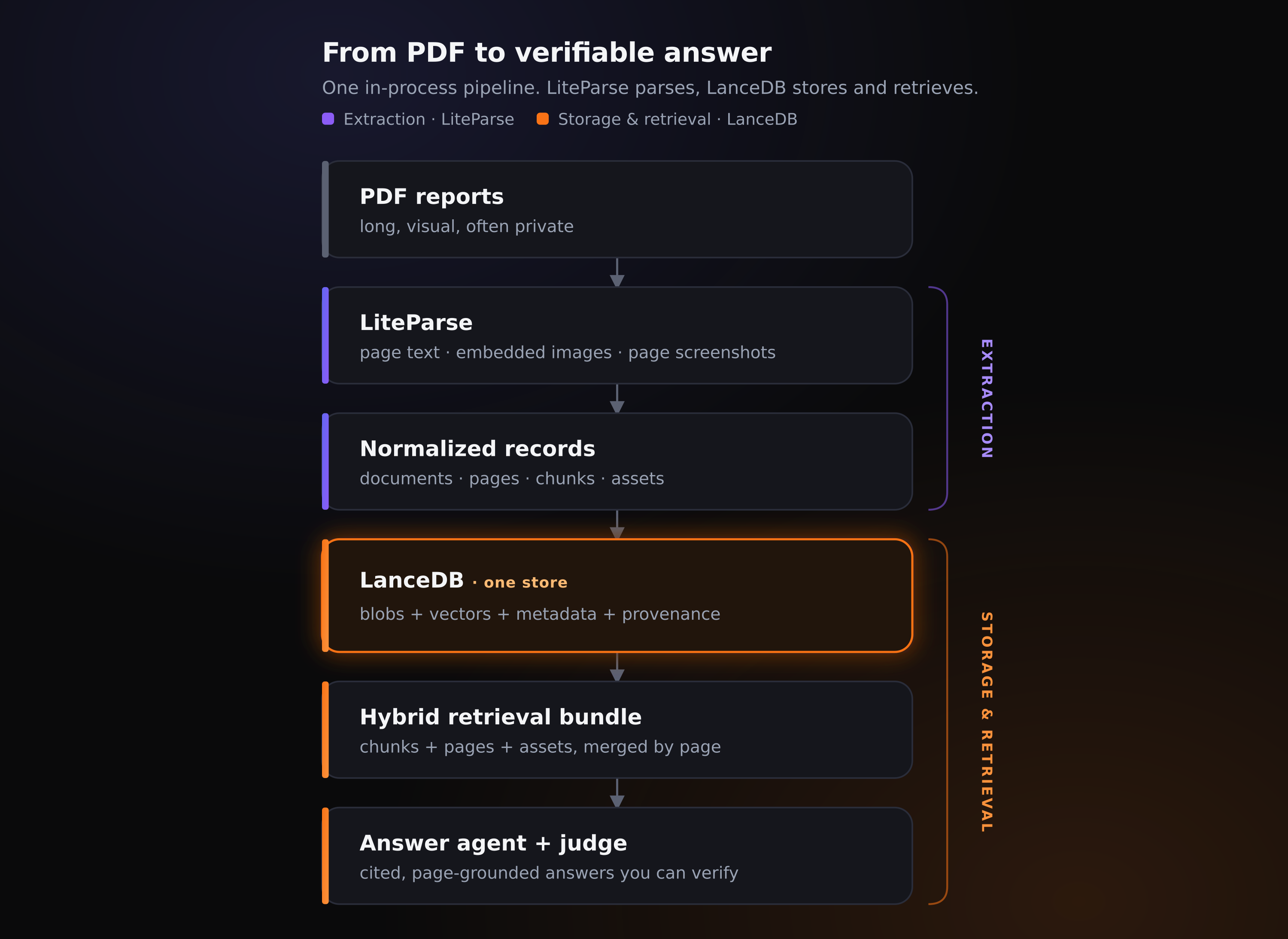
In this post we’ll build that local, inspectable evidence store with LlamaIndex’s LiteParse library for extraction and LanceDB for multimodal storage and retrieval. We’ll describe how the end-to-end pipeline works and evaluate retrieval results from an agent.

The pipeline we build looks like this:

The dataset: six ESG reports, fifty labeled questions

To keep the rest of the post concrete, we’ll use a small subset of Climate Finance Bench, an open benchmark of corporate sustainability reports paired with questions that are each labeled with the page holding the answer. We pulled six reports from well-known companies, with fifty questions in all. They make for a good stress test: the reports run from 41 to 200 pages, mix long stretches of narrative with dense tables and charts, and the questions ask for specific facts rather than broad summaries.

Each question is also tagged with the single modality of evidence it needs: text, a table, or a figure. Of the fifty, 29 can be answered from text alone, 14 require reading a table, and 7 require a figure. This split is important: the table and figure questions are exactly where text-only retrieval tends to fall apart. Here’s one of those figure questions, with its answer labeled to a single page:

{
  "question_id": "NVIDIA_Q7",
  "question": "What is the company's total carbon footprint (Scope 1, 2 and 3 emissions, in tCO2e) for FY2024?",
  "expected_pages": [12],
  "required_modality": "figure",
  "difficulty": "medium"
}

To keep things simple for this post, we parse only the pages the benchmark has labeled: 70 across the six reports, rather than all 611. This keeps each iteration fast while we tune parsing, chunking, and retrieval. However, if you want to reproduce this work, the pipeline is identical for the full document set: parsing everything just means running with --pages all instead of --pages labeled, which is what you’d do in production.

Parsing the reports with LiteParse

In an earlier post about LiteParse, we paired it with LanceDB through its TypeScript SDK. LiteParse now ships a native Python SDK on the same Rust core, and that’s what we’ll use here, since the rest of our pipeline (embeddings, storage, retrieval) runs in Python through LanceDB.

LiteParse is an open-source document parsing library that parses text with spatial layout information and bounding boxes. It’s built on a Rust core and runs entirely on a local machine with no cloud dependencies, no LLMs, and no API keys. It deterministically reads the PDF’s own text and can also read the page’s geometry directly to reconstruct the reading order from where each piece sits.

Using it from Python is straightforward. We configure one parser and then make two calls (one for parsing and another for extracting page screenshots):

from liteparse import LiteParse

parser = LiteParse(
    ocr_enabled=False,       # born-digital PDFs already have a text layer
    dpi=150,                 # enough to keep screenshots legible without bloating blob size
    image_mode="embed",      # pull embedded figures out as raw bytes
    target_pages="2,4-6,8",
)

result = parser.parse("report.pdf")        # text, positioned text_items, figure bytes
screenshots = parser.screenshot("report.pdf", page_numbers=[2, 4, 5, 6, 8])

Under that high-level interface, LiteParse hands back a small set of typed primitives. parse() returns a ParseResult: a list of ParsedPage objects, each with the page’s full reading-order text plus TextItems that keep their string, bounding box, and font. Asking for embedded images (image_mode="embed") adds ExtractedImages with raw figure bytes, and the separate screenshot() call returns ScreenshotResults with full-page PNG bytes.

Because our ESG reports are born-digital, we can keep OCR off (ocr_enabled=False), so LiteParse reads the existing text layer through PDFium rather than rendering each page and running Tesseract for OCR. It also records a bounding box for every TextItem, the exact region a span of text occupies on the page. This positional detail is what powers visual citation use cases downstream: highlighting a matched region right on the rendered page. We don’t retrieve on bounding boxes in this post, so we don’t carry them into the LanceDB tables; our retrieval uses text, figures, and screenshots. LiteParse returns them on every parse, though, and we keep the raw parse output on disk (in liteparse.json), so the option is there if we want it later.

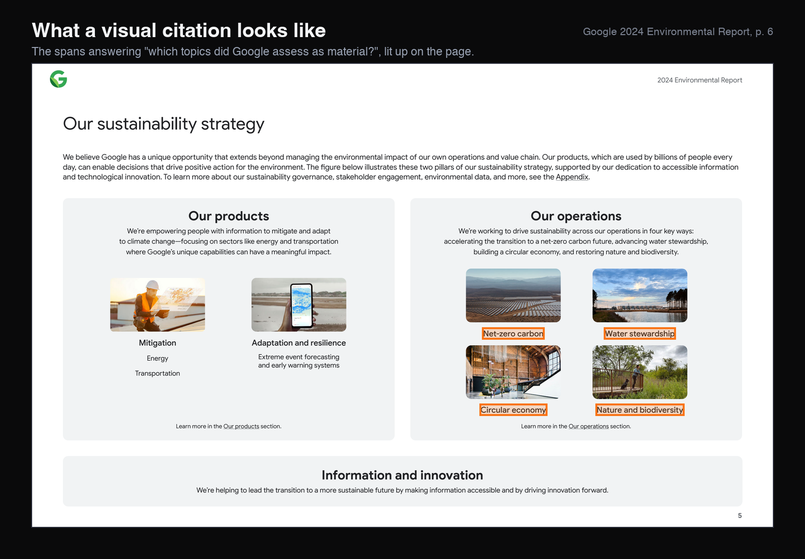
The image below makes this concrete as a visual citation. We took the page from Google’s 2024 Environmental Report that answers one of our benchmark questions, “which topics did the company assess as material?”, and lit up in orange the four spans that actually answer it, drawn straight from their TextItem bounding boxes.

Producing all of that structure (text, bounding boxes, figures, and screenshots) is cheap. Running the two parse() and screenshot() calls across our 70 labeled pages finishes in roughly 2 seconds:

The timing numbers show how fast LiteParse really is in practice: it took just half a second for parse() to pull the text, bounding boxes, and embedded figures from all 70 pages, and a little under two seconds to render the screenshots, all on a laptop with no LLM API calls. For each report, the parse step writes a small, inspectable bundle to disk: the structured parse result as JSON (pages with their text and bounding boxes), the extracted figures and page screenshots as PNG files, and a set of normalized records that tie everything back to its page.

These parsed records are the raw material we’ll use next, turning them into LanceDB tables.

Storing the evidence in LanceDB

With the reports parsed, the focus shifts to storage: getting text, images, metadata, and embeddings into one place, so we can retrieve them without stitching several systems together — we’ll do that in LanceDB. Three decisions shape how it’s laid out: the key that ties every record together, the table schema that holds text, blobs, and vectors together, and how we index and query it.

Make page identity the join key

LiteParse hands us text, figures, and screenshots as loose pieces. The decision that ties them together is to treat page identity as the common key: every record we create is stamped with the page it came from, along with its document and source. We build each page’s id during normalization, pairing a document slug (from the report’s company, year, and filename) with the real PDF page number LiteParse reports, and every other record hangs off it:

page_id  = f"{doc_id}:p{page_num}"      # nvidia_fy2024:p2  /  google_2024:p6
chunk_id = f"{page_id}:c{chunk_index}"  # nvidia_fy2024:p2:c0  /  google_2024:p6:c0
asset_id = f"{page_id}:asset:{name}"    # nvidia_fy2024:p13:asset:image_p13_0  /  google_2024:p6:asset:image_p6_0

The evidence is stored at three granularities, each record carrying the page_id it belongs to:

1. Pages hold the full page text and its screenshot.
2. Chunks are page-bounded slices of that text (about 1,200 characters with a small overlap), so a chunk never straddles two pages.
3. Assets are the visual pieces: the figures LiteParse extracted and the page screenshots.

These granularities live in separate tables in LanceDB. The best evidence for a question is often spread across multiple tables: the exact sentence in a chunk, its context in the page, the figure in an asset. Because every record carries page_id, we can search each table on its own and then, in our own code, merge the hits that land on the same page into one result with that page’s full evidence attached. This is the main reason for building the page identity keys shown above.

The schema: text, vectors, metadata, and blobs in one store

LanceDB is well-suited for this kind of data and the task at hand. A single table holds the structured columns (ids, company, page number), the full page text, the raw image bytes, and the embeddings, and it carries the indexes and version history along with them. There’s no separate object store location for the screenshots, metadata database for the provenance, or vector database for the embeddings: keep everything in one place, queried in different ways.

The LanceDB store has five tables in all. The three evidence granularities from the previous section each get their own table (pages, chunks, assets), joined by two supporting tables: documents, which holds report-level metadata, and eval_questions, which holds the benchmark we score against.

Under the hood, Lance uses Apache Arrow’s type system, and we declare each table’s schema using PyArrow. We embed text with OpenAI’s text-embedding-3-small and images with OpenCLIP ViT-B-32, which is what sets the two vector widths (1536 and 512) in the snippet below.

pages_schema = pa.schema([
    # ... ids, company, page_num, text ...
    pa.field("screenshot_blob", pa.large_binary(),           # the rendered page image
             metadata={b"lance-encoding:blob": b"true"}),
    pa.field("text_vector",  pa.list_(pa.float32(), 1536)),  # text embedding
    pa.field("image_vector", pa.list_(pa.float32(), 512)),   # CLIP image embedding
])

The lance-encoding:blob marker tells Lance to store the PNG bytes out of line, outside the normal column pages, leaving just a small (position, size) descriptor in the row. So search scans only those lightweight descriptors, and the full image bytes are fetched separately, on demand, for just the handful of pages we actually retrieve.

The two image-bearing tables are split on purpose. pages is what the retriever we benchmark later in this post runs against: each row pairs a page’s text with its screenshot and text + image embeddings. assets is more image-centric, holding the extracted figures and their image embeddings — our benchmark uses it only lightly, but it’s kept there because it’s exactly what a VLM-based agent would want if it were reasoning over the figures directly later on.

The real takeaway is that schema design depends on whatever retrieval logic you plan to run downstream, so it’s worth keeping the shapes you might need on hand: a different agent would potentially benefit from a different set of tables.

Because LanceDB is built on the Lance format, the indexes we build (covered next) live in the same store as the data, and every write produces a new version of the table, so we can inspect or reproduce an earlier state of the evidence.

Ingestion, indexing, and footprint

Ingestion and indexing are fast, completing in ~0.2 s. For this example, we created scalar BTree indexes on the columns every search filters on (company and source_pdf), and a full-text search (FTS) index on text. For small datasets of <100K rows, a vector index isn’t necessary in LanceDB — an exact nearest-neighbor search returns just as quickly here.

The part worth noticing is the size of the page images and where they end up. In a traditional setup they’d sit in a separate object store, decoupled from the text and metadata and outside any versioning. Here, the same ~100 MB of page screenshots (PNG files) are stored within the same ~101 MB pages table as their text and vectors, with almost no storage overhead. All data and indexes are versioned together, and a page’s text and its image both come from the one store, with no round trip to a separate object store or metadata service, which keeps latency down when an agent needs them.

You can learn more on how Lance manages blobs at scale in our blog post on Lance Blob V2.

Retrieval: building the hybrid bundle

Querying the data involves bounded vector search that’s scoped to a single ESG report by a company and source_pdf prefilter. We study five distinct retrieval modes:

• chunks, pages, and assets each run a text-vector search over their own Lance table
• images embeds the question with CLIP and searches the page and figure image embeddings instead
• hybrid_bundle fuses the three text searches into one page-ranked list

The hybrid bundle runs the chunk, page, and figure searches concurrently and combines their results into one ranked list of pages, keyed by page_id. It helps because the answer to a question might surface as a precise sentence in a chunk, as the whole page’s text, or in a figure’s caption, and no single search reliably catches all three. Pooling them gives each page several independent chances to rank, and merging by page then collapses the duplicates so one result carries that page’s full evidence.

To answer, we hand the agent the page pixels by reading them straight from LanceDB’s blob column:

# pull full page images for just the retrieved rows, addressed by row
rows = pages.to_lance().read_blobs("screenshot_blob", addresses=row_addresses)
images = [payload for _addr, payload in rows]

read_blobs is Lance’s API for complete payloads: it materializes the full PNG for only the handful of rows we retrieved, addressed by row, instead of scanning those bytes during search or reading loose files off disk.

Put together, the loop turns a question into an answer backed by the exact page it came from:

In practice, combining results from multiple searches is often the difference between landing the right page and just missing it. The caveat with our hybrid bundle approach is that the merge ranks purely by vector distance, so it’s a “recall-oriented fusion” rather than true reranking. It casts a wide net well, but doesn’t really sort the survivors by relevance. Using a reranker can potentially improve the results.

Does the storage layout pay off?

In this section, we build a deterministic retriever, with no agent in the loop yet. The purpose of this step is to serve as a sanity check to see whether the right pages are even returned. A “hit” means an expected evidence page showed up in the top 5 results, so the numbers below score page identity, not answer correctness.

We define the following four metrics:

Running all five retrieval modes over the fifty questions, with an OpenAI text-embedding-3-small for text and OpenCLIP for images, produces the following results:

The hybrid bundle leads on every page-finding metric, and it does so based on the schema we designed explicitly upfront. Because every record carries a page_id, the bundle can pool hits from chunks, pages, and figures and let each page win on its strongest signal. This way, rather than relying on a powerful embedding model, the schema (and the way the data is laid out) did most of the work.

Modality hits are the highest when using pages (0.94) and images (0.90) modes — these reliably return page or image evidence for the table and figure questions, where hybrid’s text-first hits fall short. images shows how searching multimodal embeddings pays off: it matches pages by image-embedding similarity through CLIP (not as well as hybrid, but solid), and even that image-vector search comes back in ~18 ms.

assets shows the weakest performance overall. This makes sense, because a figure’s caption says very little about the contents of the figure itself, so the query and the figure caption are likely not a good match in most cases. Because a figure’s real value is visual, the image vector captures it much better, but a better approach would be to combine image-based similarity search with the caption at the retrieval layer for better results on these types of queries.

The real takeaway from this sanity check study is that no single mode is universally the best. But our page-keyed layout (extracted by LiteParse and stored in LanceDB) makes it simpler to quickly test out a variety of retrieval methods.

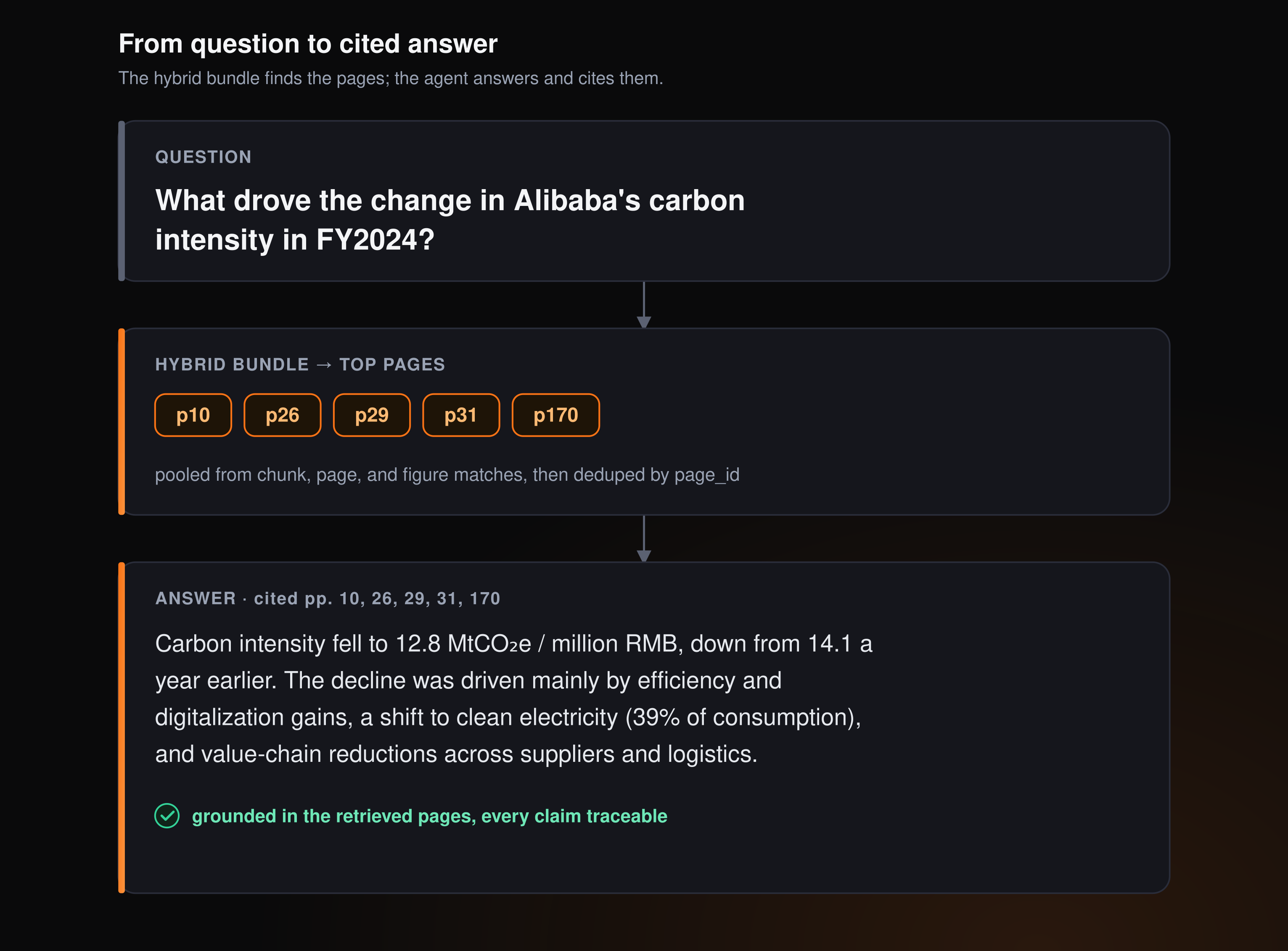
From evidence to answers: a minimal agent loop

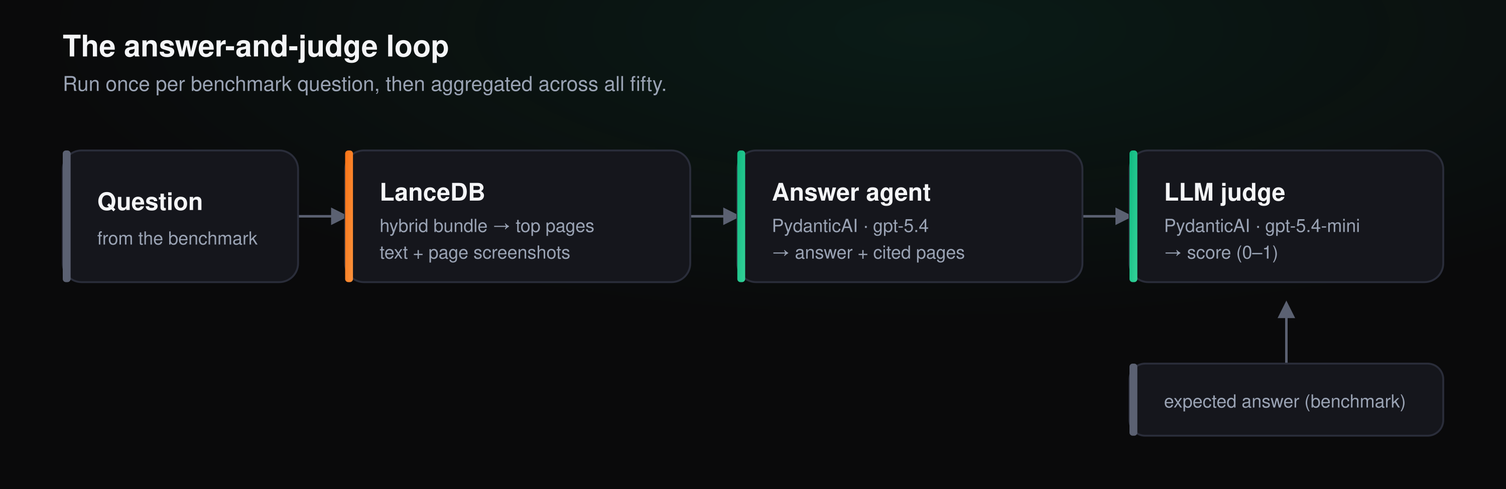
If the evidence store is built right, a thin agent layer on top should be able to use it without much ceremony. For each question in the benchmark, we retrieve the hybrid bundle and then hand a PydanticAI agent harness the result. We used gpt-5.4 as the answering model, passing it the question, the retrieved text, and the top-3 page screenshots read straight from LanceDB. It returns a structured answer along with the pages it cited and a confidence. A second model, an LLM judge (gpt-5.4-mini), compares that answer to the benchmark’s expected answer and scores it from 0 to 1.

Run over all fifty labeled questions, the agent answers 74% correctly as judged by the LLM. Table questions are the weakest, which tracks with how we parse them: a grid flattened into a run of numbers is the hardest thing for the model to reassemble.

That 74% sits just under the 82% any page-hit rate the hybrid bundle posted in the last section, and the gap between the two is informative. Getting the right page in front of the model is the retrieval layer’s job, and our LanceDB implementation here does that quite well (with plenty of room for further improvement). However, turning the retrieved context into a correct answer is the agent’s job. This agent harness we built was very simple, but more sophisticated harnesses can approach the retrieval problem from different angles, depending on the kinds of questions being asked.

What this stack enables

LiteParse and LanceDB pair well because of their shared philosophy: fast, embedded, local, while making it straightforward to keep sensitive data on your own machine. For a laptop-scale corpus this is the whole stack, but when parsing, storage, and query workloads reach production scale, both pieces have a managed path built for those scenarios: LlamaParse for AI-ready document parsing at scale, and LanceDB Enterprise for the multimodal lakehouse that can store and query the data. Design the evidence layer once, test it locally on real data, and carry the same design into production.

One piece of LiteParse’s output we didn’t touch in this post is the bounding box it records for every text item, sitting in liteparse.json. It’s possible to promote those boxes to columns on the pages and assets tables in LanceDB, and an agent app can do more than just cite pages in plain text: it can visually highlight the exact sentence or figure an answer came from, right on the rendered page. For ESG audit work, where every number gets checked thoroughly, that kind of visual citation is often what separates a demo from something an analyst will trust.

A lot of RAG pipelines tend to fall short on PDF retrieval, because they attempt to retrieve results from single searches over large chunks or entire pages at once. PDFs require approaches more nuanced than that, because they pack information in layers. Separating those layers during extraction, storing them in a way that’s suited to the retriever’s needs, and combining multiple retrieval strategies tends to produce the best results.

With modern coding agents at your fingertips, all you need to do is express your desired goals, point them to the raw data, and aid them with relevant agent skills: the effective-liteparse skill provided by LlamaIndex, and the LanceDB skill provided in the accompanying repo. Together, these help you go from raw data → working implementation quickly while writing idiomatic, clean code.

Give LiteParse and LanceDB a try for your next PDF parsing project, and check out the additional resources below.