Scalable Feature Engineering on Multimodal Datasets

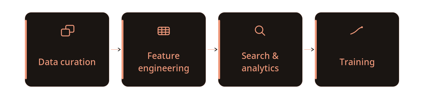
In the previous post, we curated a multimodal dataset down to a versioned table: filtering, searching, deduping, and sampling until we had the rows worth keeping. The next step is feature engineering, whose purpose is to define, extract, and transform raw data into useful information and features for your AI applications. Let’s recall the key steps in the ML data lifecycle that LanceDB is built for:

Computing features themselves, on paper, is relatively simple (all it takes is writing a transformation function that operates on existing or new data). What’s far harder, however, is everything else around that function: applying the function on all rows of the table, avoiding drift from the rows they derive from, handling failures, and how to tell later what exact version of a function produced a given column.

The focus of this post is the feature engineering piece in AI data pipelines, and the way LanceDB (and the Lance format) are built to handle it at scale. We’ll work through some of the common problems while looking at some code snippets, starting with the simplest features and building up to the ones that need some serious compute.

What this usually looks like today

Before getting to what LanceDB does differently, it helps to look at how feature engineering on multimodal data is usually done. A typical stack spreads the pieces across systems:

• Raw images and videos sit in object storage (S3, GCS, or similar).
• Metadata and derived feature columns live somewhere else: Parquet or Delta/Iceberg tables, a warehouse, or a dedicated feature store.
• Embeddings (along with a copy of the metadata that’s stored elsewhere) go into a vector database.
• Computing missing values in new columns (i.e., “backfills”) runs as a separate job through Spark, Ray, Airflow, or custom scripts.
• Provenance (the record of what produced a column) is scattered across job configs, git commits, JSON logs, and experiment tracking scripts.
• Partial failures are handled by whatever checkpointing and rerun logic each job happens to implement.

The arrangement above has a cost. A feature ends up living far from the full picture of the record it describes, drifting from the source data as it changes or evolves. Adding or recomputing a single small column can mean rewriting a large table or maintaining a side table keyed back to the original. Training and search jobs have to join across storage systems to assemble into a row. It’s hard to trace the lineage of transformations over time. A model-backed backfill job that fails three-quarters of the way through is expensive to resume, because nothing tracked which rows already finished.

Next, let’s view this through the LanceDB lens: where a feature is just another versioned column on the same table as the data it’s derived from.

What we mean by “data evolution”

Most table formats and databases handle one kind of growth well: appending rows. You collect more data, you write more records. Feature engineering grows a table the other way, by adding columns. That’s where many traditional table formats struggle, since a new column can result in the entire table (or large parts of it) being rewritten into a fresh layout. Recall that a Lance table, on the other hand, is designed for two-dimensional growth:

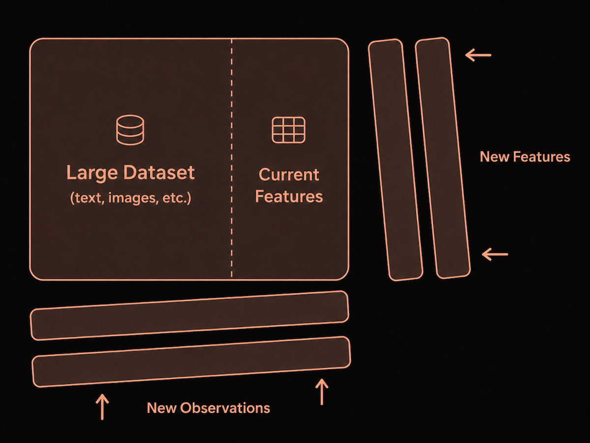
New observations arrive as new rows. New features arrive as new columns, written alongside the data that’s already there. Adding a column in Lance and backfilling it is as routine as adding a row − it’s more than “schema evolution”. It’s data evolution.

The most important point to note here is what doesn’t happen when you add a column. Lance writes only the new column’s data − the existing large blobs, captions, embeddings, metadata, and indexes remain untouched. Every write operation creates a new fragment and commits a new table version that records the change. At a later time, a compaction operation can be run to keep fragment sizes reasonable such that future read queries don’t need to touch too many fragments.

Due to this design, backfilling a new feature column in Lance that’s a few MB in size, only writes a few MB of data, even when the original table it joins is already terabytes or petabytes in size (very common with large multimodal datasets, especially when videos are involved). If you’re curious about the storage layer design that enables cheap data evolution at scale, our earlier blog post on designing a table format for ML workloads goes deep into the topic.

From the perspective of an AI engineer using LanceDB, all of this functionality is available using the same, familiar LanceDB API that reads from the table, so there’s no need to worry about elaborate decision-making about read vs. write trade-offs or complex schema migrations during the feature engineering stage.

Feature engineering adds signals to your dataset

A feature can be a derived column from data that already exists in the table, for example, caption_length from the caption, or aspect_ratio from the stored width and height. But plenty of features depend on more than the existing row itself. Some come from a model whose weights live outside the dataset (a quality score, a fresh embedding); some aggregate across many rows (the size of the near-duplicate cluster an image falls into); some join in values from a separate table.

The table below shows some common patterns used to create new features, with examples in later sections.

Each of the above adds data to a new column and attaches it to every row in the table. But because writes to a Lance table are automatically versioned, adding new features doesn’t cause governance drift the way manual file or metadata management does.

Feature engineering in LanceDB OSS

We’ll use the LAION-1M dataset that’s on the Hugging Face Hub in Lance format. Open it directly over an hf:// URI without needing to download the full dataset locally.

import lancedb

db = lancedb.connect("hf://datasets/lance-format/laion-1m/data")
table = db.open_table("train")

print(table.count_rows())
# 1,162,252 rows in total
print(table.schema)

## --- Prints the table schema ---
# image_path: string
# caption: string
# NSFW: string
# similarity: double
# url: string
# key: string
# status: string
# error_message: null
# width: int64
# height: int64
# original_width: int64
# original_height: int64
# exif: string
# md5: string
# img_emb: fixed_size_list<item: float>[768]
#   child 0, item: float
# image: binary

This single table contains 1.1M records with everything we need in one place: the raw image bytes, the caption and other text metadata, the width/height dimensions, and a 768-dimensional img_emb embedding. Feature engineering will add new columns right next to the existing columns.

To add new feature columns we’ll keep a small local copy to write against. A 5,000-row subset is plenty to demonstrate the workflow and keeps every write local and fast.

# Read the first 5,000 rows via the underlying Lance dataset scanner
subset = table.to_lance().scanner(limit=5000).to_table()

local_db = lancedb.connect("./laion-subset")
table = local_db.create_table("train", subset)

print(table.count_rows())  # 5000
print(table.version)       # 1

Add simple features with SQL expressions

LanceDB OSS can add a column straight from a SQL-style expression over fields already in the table, so the whole feature definition is a string. Let’s add three to the local table at once: caption_length, aspect_ratio, and image_area.

print(table.version)            # 1
print(len(table.schema.names))  # 17

table.add_columns({
    "caption_length": "length(caption)",
    "aspect_ratio": "CAST(width AS DOUBLE) / CAST(height AS DOUBLE)",
    "image_area": "width * height",
})

print(table.version)            # 2
print(table.schema.names[-3:])  # ['caption_length', 'aspect_ratio', 'image_area']

When you specify a SQL-like expression to add_columns as above, the table moves from version 1 to version 2 and picks up three new fields, and the computed values exist and are versioned in the same table as the columns they derive from. They’re durable and queryable like any other column, so we can use them straight away, including combining them in a single filter:

preview = (
    table.search()
         .where("caption_length > 80 AND image_area >= 512 * 512")
         .select(["key", "caption_length", "aspect_ratio", "image_area"])
         .limit(5)
         .to_polars()
)

print(preview)

shape: (5, 4)
┌───────────┬────────────────┬──────────────┬────────────┐
│ key       ┆ caption_length ┆ aspect_ratio ┆ image_area │
│ ---       ┆ ---            ┆ ---          ┆ ---        │
│ str       ┆ i32            ┆ f64          ┆ i64        │
╞═══════════╪════════════════╪══════════════╪════════════╡
│ 208260309 ┆ 158            ┆ 1.90625      ┆ 281088     │
│ 185120077 ┆ 99             ┆ 1.799479     ┆ 265344     │
│ 185120148 ┆ 181            ┆ 1.848958     ┆ 272640     │
│ 185120216 ┆ 146            ┆ 1.78125      ┆ 262656     │
│ 185120350 ┆ 115            ┆ 0.562225     ┆ 262272     │
└───────────┴────────────────┴──────────────┴────────────┘

The filter query above fetches long captions on reasonably large images, matching 35 of the 5,000 rows in the subset. This is the immediate payoff of features-as-columns: a training or evaluation job can filter on caption_length and image_area directly at read time, with no separate feature lookup and nothing to recompute, because the values are already part of the row.

Add custom features with Python functions

Sometimes, it makes sense to write a Python function for custom logic. For example, has_watermark_terms could be a flag we compute for captions that name common stock-photo sources, and can be written as a regular expression.

We write the logic as a function over a PyArrow record batch and hand it to add_columns, which maps it across the table in batches:

import pyarrow as pa
import pyarrow.compute as pc

# Takes a batch of the input columns, returns the new column
def add_watermark_terms(batch: pa.RecordBatch) -> pa.RecordBatch:
    flags = pc.match_substring_regex(
        pc.utf8_lower(batch["caption"]), "watermark|shutterstock|alamy|getty"
    )
    return pa.record_batch([flags], names=["has_watermark_terms"])

# Drop to the underlying Lance dataset to map the function over the table in batches
table.to_lance().add_columns(
    add_watermark_terms,
    read_columns=["caption"],   # only this column is read into each batch
    batch_size=256,             # rows per batch
)

add_columns reads only the caption column, runs the function batch_size rows at a time, and commits a single new table version. Nothing is loaded into memory all at once, and the existing columns are left untouched. The new column can be queried immediately:

table = db.open_table("train")
print(table.version)  # 3

flagged = (
    table.search()
         .where("has_watermark_terms")
         .select(["key", "caption", "has_watermark_terms"])
         .limit(3)
         .to_polars()
)
print(flagged)

shape: (3, 3)
┌───────────┬─────────────────────────────────┬─────────────────────┐
│ key       ┆ caption                         ┆ has_watermark_terms │
│ ---       ┆ ---                             ┆ ---                 │
│ str       ┆ str                             ┆ bool                │
╞═══════════╪═════════════════════════════════╪═════════════════════╡
│ 208260028 ┆ two young asian business woman… ┆ true                │
│ 208260261 ┆ NEW YORK, NY - APRIL 28:  Cam … ┆ true                │
│ 208260271 ┆ Nap York: offers sleep pods fo… ┆ true                │
└───────────┴─────────────────────────────────┴─────────────────────┘

20 of the 5,000 captions in the subset show watermarks. On a single machine, for a cheap function over a few thousand rows, this manual approach is perfectly fine.

Flexible data evolution in action

Earlier we described how adding a column in Lance only writes that new column’s data, while leaving existing data untouched. Let’s look at why this matters in practice. LanceDB keeps all data files (*.lance) under the laion-subset/train.lance/data directory, so we just list those files before and after the three simple features are added, and tag each one:

import os

def data_files(table_path):
    d = os.path.join(table_path, "data")
    return {f: os.path.getsize(os.path.join(d, f)) for f in os.listdir(d) if f.endswith(".lance")}

path = "laion-subset/train.lance"
before, v0 = data_files(path), table.version

# Run feature engineering here
table.add_columns({
    "caption_length": "length(caption)",
    "aspect_ratio": "CAST(width AS DOUBLE) / CAST(height AS DOUBLE)",
    "image_area": "width * height",
})

after = data_files(path)

print(f"version {v0} -> {table.version}")
for name, size in sorted(after.items()):
    state = "unchanged" if before.get(name) == size else "new"
    print(f"{size:>13,} bytes  {name[:18]}…  ({state})")

version 1 -> 2
  379,009,312 bytes  101101011000100101…  (unchanged)
      100,590 bytes  111000111110111000…  (new)

The original 379 MB data file (image bytes, embeddings, captions, and metadata) is there with the same name and the same byte count: it wasn’t touched. Three new columns went into a single new *.lance file of about 100 KB, growing the dataset by less than 0.03%, all while only writing new data and leaving existing data files untouched. This scenario is extremely common in feature engineering, which is why the storage layout used by Lance matters.

At petabyte scale, this design is all the more relevant: the I/O burden of every new column written is proportional to just that column’s values, not the size of the table itself. The storage layer decides how to write only what's needed. At a later stage, compaction can rewrite fragments to optimize the storage layout to keep query times optimal, but as a user, you focus is purely on defining the transformations (the system handles the rest),.

Where manual backfills break down

The manual path above is fine when the feature is cheap and the data/compute fits on one machine. But let's look again at what just happened: the Python function ran on a single CPU, one batch at a time. For a regex over 5,000 rows, that costs almost nothing.

Now make the feature using a model (an image-captioning or object-detection pass) on a table with hundreds of millions of rows, and that same outline needs to become a distributed job, with all the complexities that entails:

• Execution: rows have to be read in batches, spread across many workers, and placed on the right hardware (a regex check just needs CPUs, but an image or video captioning model needs GPUs).
• Robustness: workers fail and instances get preempted, so a job that dies at 80% completion shouldn’t have to restart from zero. You need checkpointing, retries, and a way to rerun only the rows still missing a value.
• Reproducibility: every worker needs the same dependencies and model weights, and months later you’ll want to know which version of the function produced a given column.

This is where the needs of storage and execution primitives clearly begin to separate themselves. LanceDB OSS already gave us the storage pieces: an evolving table with cheap column adds, no rewrites, and versioning baked in. What’s left is running the expensive computation itself across machines without hand-building the batching, retries, and checkpointing.

UDFs as an abstraction

Geneva, the feature engineering package available with LanceDB Enterprise, removes the need to build that batching, retry, and distribution machinery yourself. You describe the per-row computation as a user-defined function (UDF), and the engine runs it across the whole column for you. The workflow can be decomposed into three steps.

First, open the same table through geneva.connect:

import geneva

db = geneva.connect("./laion-subset")
table = db.open_table("train")

Next, write the feature as a UDF. Rather than a for loop over the rows, you write only the body of that loop, the part that turns one row into one value, and decorate it with @udf:

import pyarrow as pa
from geneva import udf

@udf(data_type=pa.bool_())
def has_watermark_terms(caption: str) -> bool:
    if caption is None:
        return False
    text = caption.lower()
    return any(term in text for term in ["watermark", "shutterstock", "alamy", "getty"])

Finally, register it as a column and backfill it:

table.add_columns({"has_watermark_terms": has_watermark_terms})
table.backfill("has_watermark_terms")

add_columns registers the column and records that this UDF produced it; backfill computes the values across the table and commits a new table version, like any other write.

The watermark check here was a cheap, CPU-bound regex. Heavier features follow a similar pattern: say you next want an image-quality score from a vision model, which runs far better on a GPU. Switching from a CPU to a GPU is one with one extra argument, with the rest of the UDF looking the same:

@udf(data_type=pa.float32(), num_gpus=1)   # this feature runs on a GPU
def quality_score(image: bytes) -> float:
    # a heavyweight model, loaded once per worker
    return model(image)

table.add_columns({"quality_score": quality_score})
table.backfill("quality_score")

The number of GPUs the model needs is the only execution detail you specify. From there, the engine spreads the backfill across the GPUs available to it. You write the feature logic, and the engine decides how to run it at scale.

The table below shows the transition between LanceDB OSS (where you manage a lot of these operations on a single machine manually) and what you get out of the box in LanceDB Enterprise.

When you’re building training or search pipelines on terabytes or petabytes of data, the real win comes from iterating on features rather than wrangling with infrastructure. LanceDB provides the primitives for engineers and researchers: simply define the transformation inside a function, run the backfill, and move on.

Version UDFs alongside the data itself

Like curation, feature engineering is also an iterative process. A new feature column is never just written once. Maybe its definition turned out too narrow, a better embedding model became available, or an old computed feature is superseded by a better one. Every change raises the same question months later: which version of the dataset did this result come from, and how did we produce that column?

Just as datasets are versioned in the Lance format, UDFs are also versioned in Geneva. Every registered UDF has the version information in its metadata, which you can easily explore as follows:

meta = table.schema.field("has_watermark_terms").metadata
print(meta[b"virtual_column.udf_name"])    # b'has_watermark_terms'
print(meta[b"virtual_column.udf_inputs"])  # b'["caption"]'
print(meta[b"virtual_column.udf"])         # b'_udfs/16da8499…'  (content hash of the UDF)

A new feature column isn’t just a new set of values slapped onto a given table − the table tracks the operation that produced it. When the function’s internal logic changes, you just re-point the column at the new UDF, rerun the backfill, and the recorded UDF automatically moves with it:

# the definition changed (say, a new watermark term); recompute every row
table.alter_columns({"path": "has_watermark_terms", "udf": has_watermark_terms})
table.backfill("has_watermark_terms")

# or, if a run left gaps, recompute only the rows still missing a value
table.backfill("has_watermark_terms", where="has_watermark_terms IS NULL")

This ability to do filtered backfills on only the subsets that need it, is what keeps iteration and experimentation cheap in LanceDB. A failed run or a new sequence of runs require just a few lines of code, and each write is tracked as a new version inside a manifest that sits alongside your dataset.

From a user perspective, this means you can ask not just “what was in my dataset?” but “when and how was this feature produced?”

Towards scalable, end-to-end AI pipelines

If your current feature pipeline is split across media storage, metadata tables, embedding stores, and batch jobs, the benefits of consolidation are all too real with LanceDB: a feature becomes another versioned column on the same dataset as the data it’s derived from. A table grows horizontally as easily as it does vertically, and every new feature is just another dataset tracked by another version. Move from a SQL expression, to a Python function, to a model-backed UDF without copying the dataset or rewriting what’s already there.

As a user, switching to LanceDB Enterprise/Geneva comes down to decisions around ease-of-use and scale-of-computation. For simple features that require small, local or batch workflows, the OSS path may be all you need. When computing features becomes non-trivially expensive and needs distributed execution, GPU placement, retries, checkpointing, and provenance, that’s what Geneva and LanceDB Enterprise are built to do: wrap the same per-row function in a @udf and hand it the backfill, without needing to manually manage the distributed compute underneath.

This keeps the whole ML lifecycle on one storage layer. Curation narrows down and isolates the subset we care about; feature engineering adds new signals so that search, analytics, and training pipelines downstream can always read exactly the columns they need. By versioning both the data and the operations that produced it, it’s straightforward to reproduce past decisions for debugging or auditing.

This post was a high-level tour of feature engineering for multimodal datasets in LanceDB. To go deeper on the design, usage, and abstractions, the feature engineering docs are a great place to get started. Try it out for yourself!

‍