Fine-tuning a vision-language model (VLM) is often viewed as purely a modeling problem: pick a base model and fine-tuning technique (e.g., QLoRA), point it at your data, and train. But once you’ve gone through this workflow end-to-end, you realize that most of the friction turns out to live one layer below, in the data pipeline.
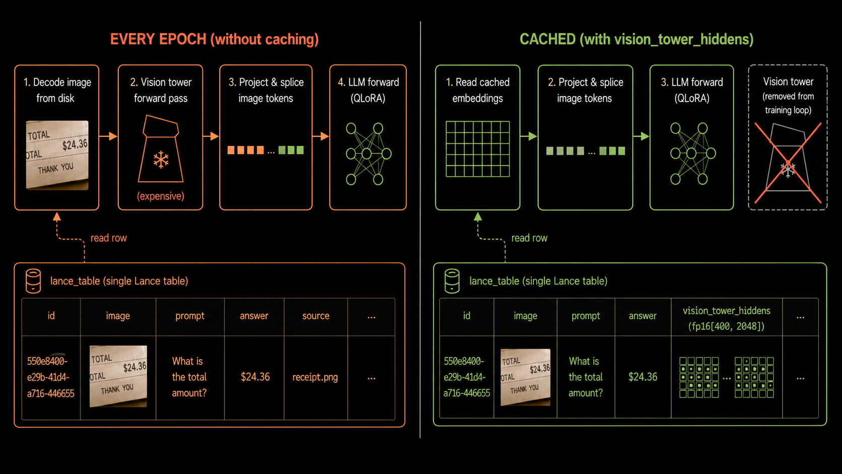
During training, two problems show up time and again. The first is wasted compute. Most pipelines recompute, on every training step, image embeddings that only ever needed to be computed once.
Those embeddings come out of the vision tower: the image-processing side of a VLM. It takes the image pixels, runs them through a vision encoder, and projects the result into the same hidden space the language model uses for text tokens. In this QLoRA setup, that vision tower stays frozen during fine-tuning, so it returns the exact same output for a given image on every epoch.
The second problem is data sprawl: in traditional pipelines, derived features get relegated to standalone files scattered around the dataset, drifting away from the rows they describe, making it hard to reliably reproduce experiments and to know what produced a given feature.
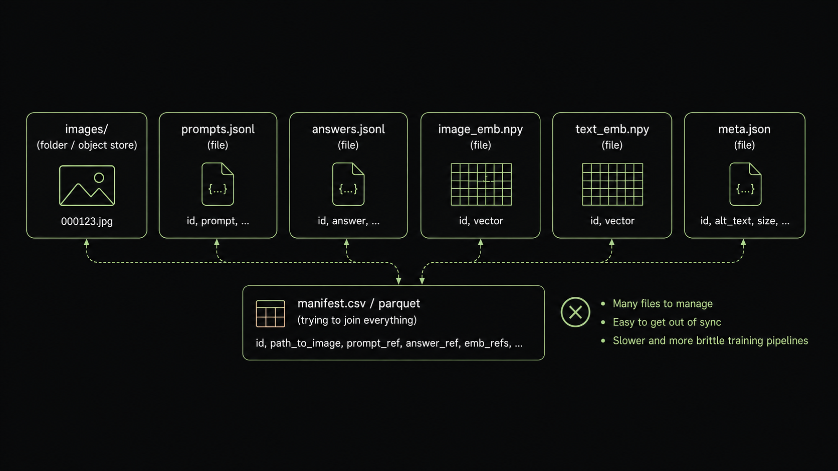
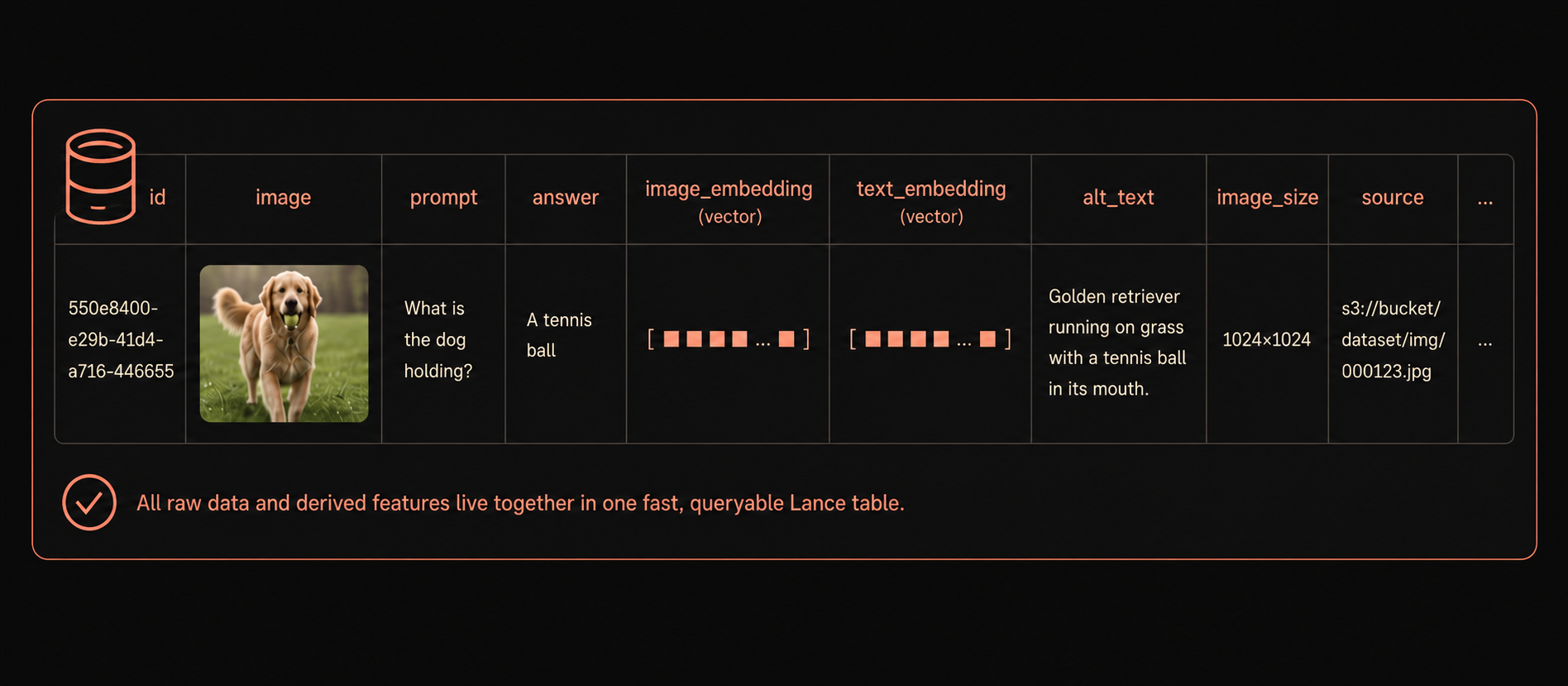
The cleaner shape is to keep the raw data and the features derived from it together as columns in place, which is LanceDB’s approach. Instead of trying to coordinate images, prompts, labels, embeddings, and metadata across separate files, every training example becomes a queryable row inside a Lance table, with the raw inputs and materialized features living side by side.
In this post, we’ll illustrate that fine-tuning a VLM is as much a data-management problem as it is a modeling one, and once we view it that way, it will become clear how the features of Lance (the format) and LanceDB (the platform) make this whole process simpler.
The key idea: Materialize the expensive part, once
The solution follows straight from the problem: if the vision tower returns the same embeddings every epoch, we should compute them once and store them. So we run each image through the vision tower a single time and write the result into a column on the same table, vision_tower_hiddens.
Our running example throughout is Qwen2.5-VL-3B, fine-tuned with QLoRA on TextVQA, a benchmark that asks the model to answer questions about text written inside an image. At that model’s 560px input size, each image reduces to 400 tokens at the language model’s hidden size of 2048, so the materialized column holds a fixed-size fp16[400, 2048] tensor per row.
With the embeddings materialized, the training loop never touches the vision tower. Instead of decoding an image and running the encoder on every step, it reads them straight off the table and splices them into the language model’s input at the image-token positions. We can drop the vision tower from the model entirely, leaving nothing in the loop but the language model’s own forward and backward pass.
While the idea above is straightforward, it might be challenging to implement using a traditional data stack. When precomputed features are scattered across flat files, a metadata database, and object storage, they’re hard to stream to the GPU fast enough to keep it sufficiently fed, and every new experiment slows down because the data is not in one place.
Lance and LanceDB provide three specific benefits, making this approach both fast and practical:
We’ll unpack these one at a time.
Benefit 1: Creating the feature is cheap
When operating over Parquet-based table formats, adding a new column means rewriting the dataset (or large parts of it), because of Parquet’s row-group design and how data is laid out on disk. For a large multimodal corpus where every row already stores image bytes, that’s an enormous amount of data to rewrite just to add on one derived feature column (that could be tiny in comparison to the full table).
To avoid this problem, teams typically leave the original data alone, write the new feature to separate files, and join everything back at load time. Even though the write stays cheap, there’s now a coordination problem to manage, which can slow down experimentation over time, as ad hoc scripts need to be written to manage and track what changed.
Lance is built for data that grows in two dimensions (rows and columns). It’s called “data evolution”. Appending a column writes only that column’s data plus a new version of the table’s manifest; the existing columns are never rewritten. The new feature lands in the same table as the data it describes, with versioning and provenance baked into the whole design.
This is the capability we need to materialize a feature column. We connect through LanceDB, open the table, and grow its schema with add_columns. For a column the database can compute on its own, we hand it a SQL expression and Lance materializes the values into a new column, leaving the existing data untouched:
import lancedb

db = lancedb.connect("data")          # directory holding the table
table = db.open_table("textvqa")

# a cheap derived column, computed in-database, no rewrite of the existing columns
table.add_columns({"question_length": "length(question)"})
The expensive columns grow the schema the same way: vision_tower_hiddens is just another column on this table, but the heavy lifting happens in a separate backfill step. That backfill can be applied manually by constructing PyArrow records in batches, and looping through the entire dataset, but Geneva (the feature engineering package that ships with LanceDB Enterprise) makes this a lot simpler, and we’ll get to it in Benefit 3.
The highlight is that Lance format makes the column cheap to add. Because the existing columns are never rewritten, raw data and all derived features live in one table. That table becomes a single source of truth for exploration, curation, training, and evaluation, with no custom metadata log to maintain and no second copy that drifts out of sync.
Benefit 2: Reading it back during training is cheap
Training use cases tend to impose punishing access patterns on the storage layer: shuffled batches of random rows, mixed in with sequential scans, every epoch. Lance handles these mixed workloads well because its fixed-size list columns store each row’s tensor at a known offset, so it jumps straight to the rows a batch wants and reads only those bytes.
Parquet, on the other hand, packs rows into large row groups, so a random batch forces it to decode whole row groups just to recover a handful of rows. To test the gap in practice, we converted two column groups to uncompressed Parquet and timed their sequential and shuffled reads against Lance:

Parquet is fastest in the one case training rarely sees: a sequential scan of the raw columns. But in the access patterns training actually uses, Lance pulls ahead. Shuffled raw batches stay fast (2,613 rows/s in Lance vs 352 in Parquet), and on the materialized fp16 vision vectors Lance is ~16x faster even sequentially (1,452 vs 90). Parquet’s fp16 shuffled read is slow enough that we skip it in this benchmark, while Lance’s holds up at 2,149 rows/s.
From the user’s perspective, this fast path is exposed through a convenient abstraction: LanceDB’s Permutation API, which lets AI engineers express shuffled, projected, random-access reads without dropping down to the format internals. We’ll put it to work when we wire up the training loop later in the post.
Benefit 3: Iterating on the feature is fast
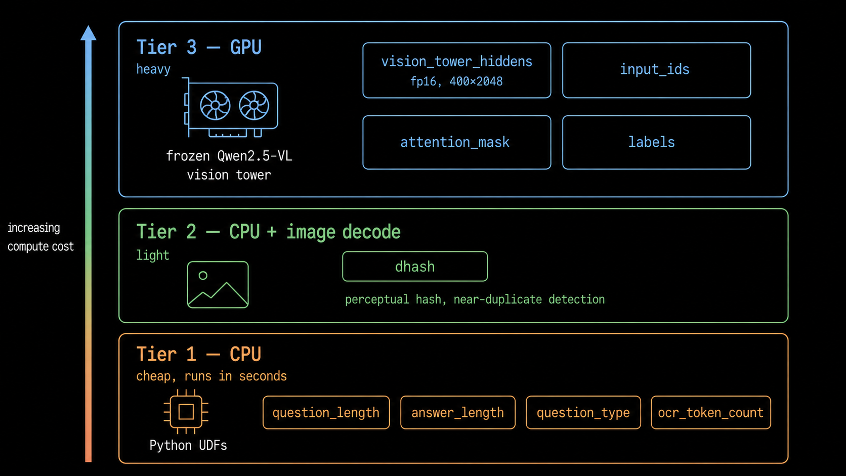
A multimodal dataset rarely stays still for long. Feature engineering work starts with something trivial like counting OCR tokens (a CPU function that runs in seconds), then grows into something heavy like running a frozen vision tower over the whole corpus on a GPU. The cheap end is easy to script, but the expensive end is where iteration slows down, because now you’re hand-rolling batching, GPU placement, checkpointing, and retries just to compute one column.
Benefit 1 showed how the Lance format makes backfilling into new columns cheap, but something still needs to compute the values. Geneva provides that engine. You define a feature as a Python UDF, and the same abstraction works whether it’s a one-line CPU function or a stateful class that lazy-loads a model onto the GPU:
import pyarrow as pa
from geneva.transformer import udf

@udf(data_type=pa.int32(), input_columns=["ocr_tokens"])
def ocr_token_count(ocr_tokens: list[str] | None) -> int:    # Tier 1: CPU, runs in seconds
    return len(ocr_tokens) if ocr_tokens else 0

@udf(data_type=pa.list_(pa.float16(), 400 * 2048), input_columns=["image"])
class VisionTowerEmbedder:                                   # Tier 3: loads Qwen's ViT on GPU
    def __call__(self, image: bytes) -> list[float]:
        ...   # decode -> frozen vision tower -> fp16[400, 2048]
To materialize a new column, we register the UDF on the table and let Geneva run the backfill across the corpus, distributing the work, checkpointing progress, and scaling concurrency so we don’t have to:
import geneva

g = geneva.connect("data")
table = g.open_table("textvqa")

table.add_columns({"vision_tower_hiddens": VisionTowerEmbedder})
table.backfill("vision_tower_hiddens", concurrency=8)
Using these patterns, you can easily define transforms from the cheap Tier 1 text columns used to curate a training slice, through a Tier 2 perceptual hash for near-duplicate detection, all the way to the Tier 3 GPU embeddings the training loop reads.
Adding a new feature means writing one function and running its backfill, not standing up a new pipeline, and that’s what keeps experiment turnaround short.
How fine-tuning is done
Let’s briefly go over the fine-tuning task that’s enabled by the steps above. TextVQA is a harder variant of conventional visual question answering: the model has to answer questions about text that appears inside the image, for example:
- The airline or brand name on a sugar packet
- The time on a phone screen
The task expects the model to actually reason over the image and its textual contents rather than just recognize the objects in it. The base model we’ll use is Qwen2.5-VL-3B-Instruct, and our goal is to improve its performance by fine-tuning it with the QLoRA method.

Keeping fine-tuning small with QLoRA
Fine-tuning a model this size the naive way means updating all of its billions of weights, which needs a matching amount of GPU memory. QLoRA gets around that on two fronts. LoRA (Low-Rank Adaptation) freezes the base model and trains only a small set of low-rank adapter matrices inserted into the language model’s attention projections, so we update a tiny fraction of the weights.
The “Q” (quantized LoRA) loads that frozen base in 4-bit precision, shrinking its memory footprint further. Together they bring a 3B vision-language model within reach of a single small GPU, around 5 GB of VRAM in this example.
From the table into the model
The vision tower stays frozen throughout fine-tuning, which is exactly why we could materialize its output ahead of time. So we take it out of the training model altogether and load only the 4-bit quantized language model with its LoRA adapters.
Each training step pulls a shuffled batch of the materialized columns through LanceDB’s Permutation API, the abstraction we mentioned in Benefit 2. It gives AI engineers a simple way to express shuffled, projected reads, while underneath it leans on everything the Lance format provides: fixed-size list columns fetched by offset and streamed to the GPU as Arrow batches, with no row groups to re-decode and no per-row Python overhead.
from lancedb.permutation import Permutation

perm = (
    Permutation.identity(table)
    .select_columns(["vision_tower_hiddens", "input_ids", "attention_mask", "labels"])
    .with_format("arrow")
)
This yields a stream of Arrow record batches, one per step. A small collate function turns each batch into the tensors the model expects, reshaping the flat vision_tower_hiddens back into [batch, 400, 2048] and converting the token columns into integer tensors:
import torch

def collate(batch):                      # batch: a pa.RecordBatch from the Permutation
    n = batch.num_rows
    vision = batch.column("vision_tower_hiddens").values.to_numpy(zero_copy_only=False)
    return {
        "vision_hiddens": torch.from_numpy(vision.reshape(n, 400, 2048)),   # fp16
        "input_ids":      torch.tensor(batch.column("input_ids").to_pylist()),
        "attention_mask": torch.tensor(batch.column("attention_mask").to_pylist()),
        "labels":         torch.tensor(batch.column("labels").to_pylist()),
    }
The last step is to put the vision embeddings where the model expects them. The prompt reserves one <|image_pad|> slot per vision token (400 per image), and we drop the materialized vision_tower_hiddens into exactly those positions before the language model runs:
inputs_embeds = model.get_input_embeddings()(input_ids)
mask = (input_ids == image_pad_id).unsqueeze(-1).expand_as(inputs_embeds)

# write the materialized embeddings into the image-pad slots
inputs_embeds = inputs_embeds.masked_scatter(mask, vision_hiddens.to(inputs_embeds.dtype))
With that, the model sees the image without ever running the encoder.
The code after that is just plain PyTorch: optimizer, gradient accumulation, checkpointing, and saving the QLoRA adapter.
loader = make_cached_loader(
    "/path/to/textvqa_colab_train.lance",
    batch_size=2,
    shuffle=True,
)

for batch in loader:
    batch = batch.to(device)
    loss = forward_cached(model, batch, image_pad_id)
    (loss / grad_accum).backward()
    ...
The training loss falls as the adapter learns from the cached features, and peak VRAM stays at 5.3 GB because QLoRA trains without keeping the vision tower active.
step  10/300  loss=2.6694  5.9 samples/s
step  20/300  loss=2.3133  6.1 samples/s
                 .
                 .
                 .
step 290/300  loss=0.0359  6.3 samples/s
step 300/300  loss=0.4750  6.3 samples/s
saved adapter to runs/colab_lora/lora | peak VRAM 5.3 GB
One training loop, end to end
What makes this loop “end to end” is that everything it touches lives in one Lance table: raw image blobs, CLIP embeddings, OCR metadata, and the derived vision_tower_hiddens and token columns. There’s no constellation of bespoke files, databases, and formats to stitch together, the kind that traditional training infrastructure usually accumulates over time.
Because the data sits in one place and in the right shape, wiring it into training is “boring” in the best way possible: the data loader and forward pass shown above are ordinary PyTorch code. We didn’t need to rewrite the training loop; we just pointed it at a Lance table. The data layer does the heavy lifting, so the model training code stays as it was.
In this end-to-end example, the fine-tuning run completed in ~15 minutes (on an H100 GPU) and the held-out curated validation split produced the following results:
Although a 2.1 pp gain is relatively modest, it serves as a proof point that the pipeline trains well end to end. Using this methodology, it’s possible to train a better base model on more data to push the gains up even further.
Takeaway: Faster training lifecycles
In this post, we demonstrated how the Lance format’s performance and the platform’s abstractions come together to compress the model training and fine-tuning lifecycle. We pre-computed features with LanceDB’s feature-engineering library, persisted them to the same Lance table as the raw data, and leaned on the performance benefits of the Lance format to keep the end-to-end loop fast.
The gains from using LanceDB aren’t purely about model performance on the task. An AI researcher can test out their ideas far more rapidly by writing out their transformation logic and letting the system handle the scale and distribution of the compute. And every one of those ideas benefits from the performance optimizations in the underlying Lance format layer, which come together in two ways: fast random access and scans on the exact kind of data training sees, and, just as importantly, cheap data evolution that lets researchers add as many new columns as they need without any full table rewrites.
If you’re an AI researcher, going from idea → implementation → validation has never been this straightforward.
To reproduce the full pipeline end to end, including the curation, exploration, and evaluation steps, dig into the resources below: