A Practical LLM Pretraining Pipeline with LanceDB

Most pretraining pipelines make several copies of the same dataset. Raw text becomes cleaned text. Cleaned text becomes tokenized text. The tokens are then shuffled, packed, and split into shards. Each step creates a new set of files. Change the tokenizer, quality filter, dedup rule, or sequence length, and you may have to rebuild everything that comes after it.

LanceDB stores the raw text, the columns we add during curation, the tokens used for training, and the data we search after training. Sequence packing happens inside the dataloader while the rows stream out.

Here is the first run from start to finish:

That is 11 minutes from raw text to training-ready data, and 25 minutes from raw text to a finished model.

Sequence packing: use all of the training data

A transformer trains on blocks with a fixed number of tokens. We use blocks of 1,024 tokens. Real documents, of course, are not all exactly 1,024 tokens long.

The simple solution is to pad short documents and cut long ones. But padding makes the GPU do work on empty space, while truncation throws away real text.

Take three documents with 300, 1,500, and 700 tokens. Padding or truncating them creates three blocks with 3,072 positions in total. Only 2,024 positions contain useful tokens. The rest is padding, and 476 tokens from the long document are never used.

Sequence packing avoids that waste. It joins the documents with an end-of-text token, then cuts the combined stream into 1,024-token blocks. The next document fills whatever space is left in the current block. Almost every position contains a real token, and long documents are not cut off.

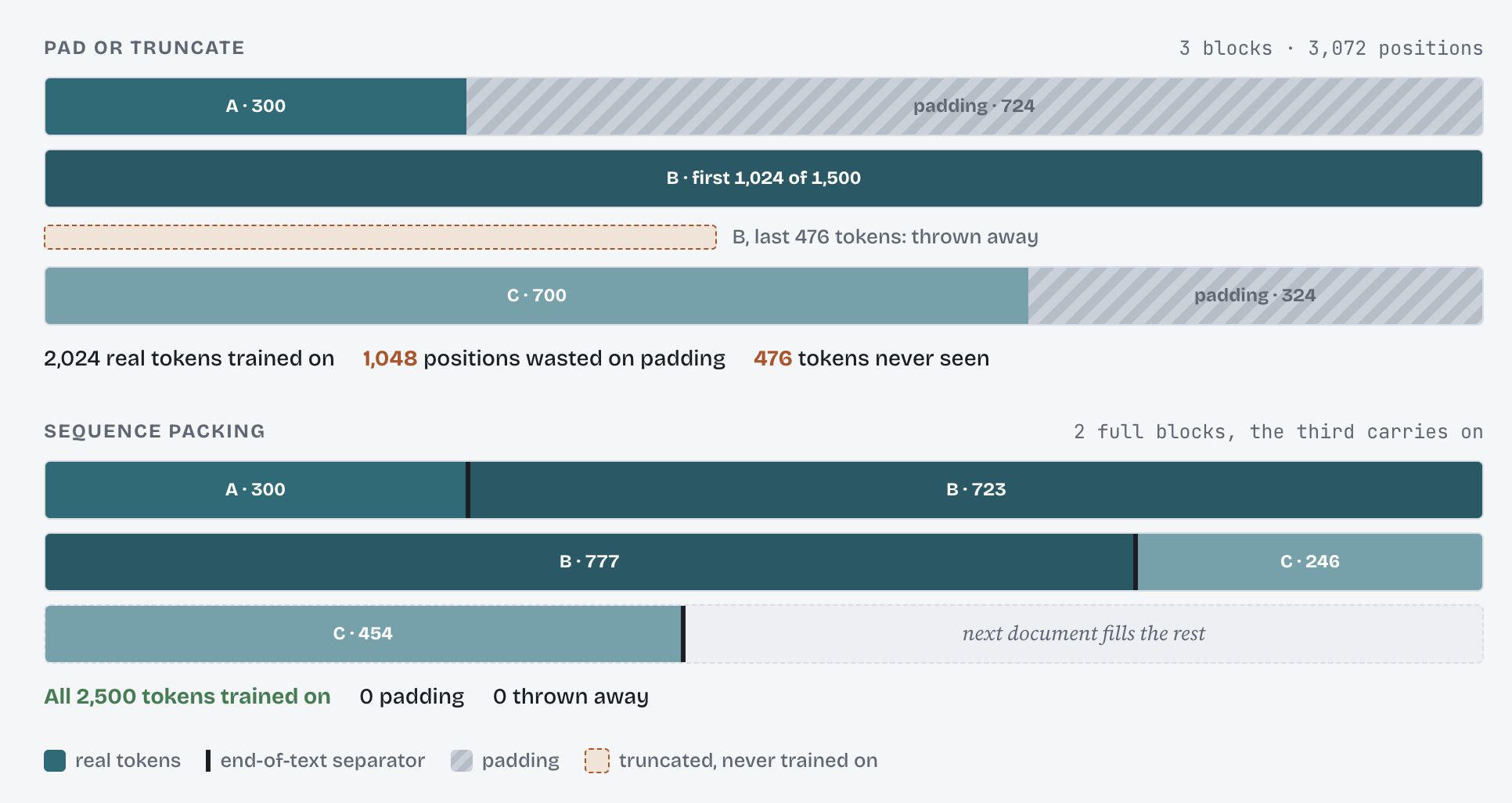
This makes a large difference on a real corpus. In the 17.5M-document dataset later in this post, padding or truncating at 1,024 tokens would keep only 61.9% of the tokens. Packing uses all of them.

Packing is often another preprocessing step. A script reads the tokens, creates fixed blocks, and writes another dataset. Change the block length or filter, and those files have to be rebuilt.

LanceDB packs inside StreamingDataset instead, while rows stream from the table:

ds = StreamingDataset(
    tbl,
    columns=["input_ids"],
    filter="NOT is_dup AND score >= 1.0 AND (id % 100 != 0)",
    num_splits=128,
    pack_sequences=1024,        # block length; turns packing on
    eos_id=tok.eos_token_id,    # separator placed between documents
    pad_id=tok.pad_token_id,    # used only if a split runs out of documents
    blocks_per_epoch=2_373_376, # exact number of blocks in one epoch
)

‍The main settings included:

• pack_sequences sets the block length and turns packing on.
• eos_id is the token placed between documents.
• blocks_per_epoch controls how many blocks the model sees in one epoch. We calculate it from the token counts already stored in the table. The loader can also estimate it when set to "auto".

Each batch contains the packed input_ids and doc_ids, which mark the document boundaries. We use normal end-of-text-separated attention, as GPT-2 does.

The loader also shuffles documents every epoch before it packs them. Change the seed, filter, or block length, and the next run changes immediately. There is no packed dataset to rebuild.

One LanceDB table for the whole pipeline

The table starts with the source data. As the pipeline runs, it gains a few new columns:

v1  ingest      id │ text │ source │ score │ n_chars
v3  curate                                          │ is_dup
v13 tokenize                                                 │ input_ids │ n_tokens

‍Every stage follows the same basic pattern: read an existing column, compute something, and write the result as a new column. Deduplication adds a true/false flag. Tokenization adds token IDs and a token count. The training process then filters and reads those columns directly.

This stays cheap for two reasons:

1. LanceDB writes only the new column. It does not rewrite the data that is already there. Adding a column creates a new table version, while the old version stays readable. Feature engineering adds only the storage cost of the new feature.
2. LanceDB Feature Engineering fills those columns in. You write a normal Python function, or UDF, that takes a column and returns a column. Geneva runs it across workers and checkpoints its progress. If the job stops, it resumes where it left off and skips rows that are already done.

The same function can run on a laptop or a cluster. If the function needs a GPU, its decorator can request one for each worker. In practice, feature engineering becomes “add a column,” and the storage cost is just the size of that column.

Deduplication is the smallest example. The first pass finds repeated text and records the duplicate row IDs. The second pass uses a backfill to write an is_dup flag:

seen, dup_ids = set(), set()
for batch in tbl.search().select(["id", "text"]).to_batches(1024):
    for rid, text in zip(batch["id"].to_pylist(), batch["text"].to_pylist()):
        h = hashlib.md5(" ".join(text.split()).encode()).hexdigest()
        dup_ids.add(rid) if h in seen else seen.add(h)

@udf(data_type=pa.bool_(), input_columns=["id"])
def is_dup(id: pa.Array) -> pa.Array:
    return pa.array([i in dup_ids for i in id.to_pylist()], pa.bool_())

tbl.add_columns({"is_dup": is_dup})  # declare the column
tbl.backfill("is_dup")               # fill it in

The same pattern works for a small feature like a flag, or a model running on GPUs.

The flag for 2.4M rows adds only 306KB:

flagged 22558 duplicate rows
data files: 3 -> 6, bytes: 5,146,223,696 -> 5,146,530,300
(+306,604 bytes for the new column; nothing rewritten)

‍The 2.43B token IDs add about 7GB, which is the size of the tokens themselves, not another copy of the original text.

Curation rules stay as filters instead of becoming new datasets:

filter="NOT is_dup AND score >= 1.0 AND (id % 100 != 0)"

The loader excludes duplicates, low-quality rows, and the held-out 1% from training. To train only on rows with score >= 3, we can update the filter without rebuilding the dataset. The held-out data is used to calculate validation loss during training.

Because the data stays in a LanceDB table, we can curate and mine the same rows with SQL, full-text search, and vector search, then write the result back as another column:

tbl.search().where("NOT is_dup AND score >= 1.0")              # SQL filter
tbl.search("photosynthesis carbon dioxide", query_type="fts") # full-text search
tbl.search(query_vector)                                        # vector search

Tokenizing the dataset

Tokenization is usually the point where raw text becomes a second dataset. It is also the first job here that needs many workers, so it is a good fit for a backfill.

@udf(data_type=pa.list_(pa.int32()), input_columns=["text"])
class TokenizeHF:
    def __call__(self, text: pa.Array) -> pa.Array:
        if self._tok is None:
            self._tok = AutoTokenizer.from_pretrained("gpt2")
        return pa.array(
            self._tok(text.to_pylist())["input_ids"],
            type=pa.list_(pa.int32()),
        )

conn = geneva.connect(db_path)
tbl = conn.open_table("corpus")
tbl.add_columns({"input_ids": TokenizeHF()})
with conn.local_ray_context():
    tbl.backfill("input_ids", udf=TokenizeHF(), concurrency=32)

‍On a 112-core machine, 32 workers tokenize 2.4M documents in under five minutes. The tokenizer loads once per worker, not once per batch. Another Feature Engineering backfill writes the n_tokens column that the packer uses to calculate the epoch size.

The job checkpoints as it runs, so it can resume after a failure. When we move to the 17.5M-document corpus later, we increase the worker count from 32 to 64. The tokenization function does not change.

At this point the same table holds the source text, curation flags, token IDs, and token counts. It is ready for training.

Training GPT-2 124M

We train a nanoGPT-style GPT-2 124M model with all common optimizations like fused QKV, PyTorch SDPA, tied embeddings, torch.compile, bf16, and DDP across 8 H100s. The global batch is 512 sequences of 1,024 tokens:

torchrun --nproc-per-node 8 train.py --model small --tokenizer hf:gpt2 \
    --pack --compile --batch-size 32 --grad-accum 2 --seq-len 1024 --epochs 1 \
    --num-splits 128 --read-batch-size 8 --io-queue-depth 1 \
    --transform-parallelism 2 --num-workers 2

‍One epoch covers 2.43B tokens in 4,636 optimizer steps:

step 1000/4635 | loss 3.9628 | 3,180,409 tok/s | mfu 34.5%
val loss @ step 1500: 3.5971
val loss @ step 3000: 3.3201
val loss @ step 4500: 3.2363
final: opt_step=4636 val_loss=3.2361

‍The run finishes in 14 minutes at 3.18M tokens per second and 34.5% model FLOPs utilization (MFU). The GPUs stay fully fed, so training remains GPU-bound rather than I/O-bound. Moving from 4 to 8 GPUs doubles throughput while keeping about the same efficiency and final loss.

The small model can produce fluent text, but its facts are weak. Here it continues the prompt “Photosynthesis is the process by which”, using the step-4,000 checkpoint at temperature 0.8:

‍Photosynthesis is the process by which photosynthetic algae, the photosynthetic algae, convert sugars to sugars.

That is roughly what we should expect from a 124M-parameter model trained on 2.4B tokens: it sounds natural, but it does not know enough.

Before comparing loaders, though, we need to make sure our own loader is fast enough to feed all eight GPUs.

Using LanceDB’s profiler to tune the loader

In our first loader test, throughput is only 158k tokens per second for one GPU’s share. At that speed, the full 8-GPU job spends too much time waiting for data.

Instead of changing settings at random, we use the queue statistics printed by the LanceDB dataloader and a controlled loader-only sweep. The training script prints the state of the loading pipeline on each log line:

epoch 0 step 1000/4635 | loss 3.9628 | 3,180,409 tok/s | mfu 34.5%
q 24264/49928/41176/31640 | fetch 168.3s | transform 15.1s

‍The four numbers after q tell us where the rows are:

1. 24,264 unscanned rows: still waiting to be read from the table.
2. 49,928 rows in the raw queue: already read and waiting to be packed.
3. 41,176 rows in the cooked queue: packed blocks that are ready for the GPU.
4. 31,640 consumed rows: already sent to training.

The exact values are less important than the overall pattern:

• If both queues are nearly empty, reading from storage is too slow.
• If the raw queue is full but the cooked queue is empty, reading is fast and packing is too slow.
• If both queues are full, the loader is ahead of the GPU. That is what we want.

The fetch and transform timers give another view of the same pipeline. This log comes from the final tuned training run. Both queues contain plenty of work, which means the loader is ahead and the GPU is the bottleneck.

A  reproduction run raising io_queue_depth from 1 to 8 grows the raw queue from 61k to 169k rows, while throughput falls by 3.7 times. The readers are not waiting on storage. At higher queue depths, they read further ahead and fill the raw queue, but overall throughput falls because they crowd the packer out of the Python interpreter lock.

These measurements come from a loader-only benchmark, with no GPU training thread or host-to-device copies in the process. The contention is inside the loader. Reader, transform, and packing threads all need the Python interpreter lock when they build Python objects. Creating too many reader and transform threads leaves less time for the serial packer to make progress. We change three settings, one at a time:

• io_queue_depth: 4 → 1. Reader thread count is num_splits × io_queue_depth. With 32 splits per process, this cuts the number of reader threads from 128 to 32 and gives the packer more time to run.
• transform_parallelism: 112 → 2. Each process uses two transform threads instead of one per CPU core.
• num_splits: 256 → 128 across the job, or 32 → 16 per process. With an I/O depth of 1, this also cuts the reader count from 32 to 16 per process.

Each change helps:

The final flags were:

--io-queue-depth 1 --transform-parallelism 2 --num-splits 128

Global shuffle from S3, without a pre-shuffled copy

We compare the original Lance corpus table with four derived formats: a Lance blocks table, MosaicML Streaming (MDS) shards, Parquet in its original order, and pre-shuffled Parquet. Every row uses the same model and machine. Only the loader changes.

The comparison column below shows throughput relative to the Lance corpus table in the same location.

Benchmark setup. We write Parquet without compression and use small 4MB row groups to help its random-read performance. Mosaic uses uncompressed 256MB shards, its own loader with 8 workers per GPU, online shuffle enabled with a fixed seed, num_canonical_nodes=8, and one shared cache per node. The derived formats start from data that is already filtered and packed, while the Lance corpus loader does that work during training.

The Lance blocks table and pre-shuffled Parquet read samples in an order that is already written to disk. Mosaic is different. It shuffles each epoch using its default py1e algorithm. This shuffles the shard order globally, then shuffles samples within a window of neighboring shards, so each batch mixes nearby shards rather than the whole corpus. It approximates a global shuffle, while the Lance corpus loader draws a fresh permutation across every document. All three stay within about 1% of the Lance corpus table on local disk.

The harder case is a fresh global shuffle. At the start of each epoch, LanceDB shuffles the documents across the whole corpus, then reads and packs them in that new order. This needs fast random reads. It also means the shuffle is not baked into the data: change the seed, filter, tokenizer, or sequence length, and there is no shuffled dataset to rebuild.

This is where the storage format matters. In the Python Parquet reader used here, a random sample reads the full 4MB row group even when the loader needs only one row. A Rust Parquet reader can narrow this to a single page, typically around 1MB. That would reduce wasted reads, although it would still read more data than the requested row. From local disk, throughput falls from about 3.17M to 2.02M tokens per second. From S3, it falls to 74k. That is 43× slower than LanceDB reading from the same bucket.

LanceDB is built for fine-grained random access, so it runs the global shuffle directly against the corpus table in object storage. It reaches 3.16M tokens per second from local disk and the same 3.16M from S3. Prefetching keeps enough random reads in flight to hide the network round trip.

That is the main difference. LanceDB gets the speed of a pre-shuffled dataset without creating one. Every epoch can use a fresh global order, while the source table stays unchanged and queryable.

MosaicML Streaming shuffles online and reaches 3.17M tokens per second from local disk. From S3, its average falls to 2.87M because throughput dips while new shards download into the local cache, reaching 0.73M in the slowest window. The shuffle is the same in both runs, so it does not explain the gap. MDS bakes in the tokenizer, filter, dedup decisions, block length, and packing, but not the shuffle order. LanceDB applies the filter, packs documents, and globally shuffles them directly from the corpus table.

Lance keeps the source data queryable. We can change a filter, add a column, inspect a row, or look up what the model saw without making another dataset.

The small-model benchmark puts heavy pressure on every loader. Next, we try the same pipeline with seven times more data and a larger model.

Scaling to 17.5M documents and GPT-2 354M

We repeat the pipeline on 24 FineWeb-Edu sample-100BT shards: 17.48M documents and 18.06B GPT-2 tokens. We then train GPT-2 medium, a 354M-parameter model, on a 7B-token budget.

Preparing the larger dataset takes 63 minutes of wall time. Training takes 97 minutes on 8 H100s, compared with 3h 06m on 4 H100s.

This is the corpus where padding or truncating would keep only 61.9% of the tokens. Sequence packing lets the model train on all of them.

val loss @ step 2000: 3.4359
val loss @ step 4000: 3.1417
val loss @ step 8000: 2.9297
val loss @ step 12000: 2.8452
final: opt_step=13351 val_loss=2.8410

The larger model passes the 124M model’s final validation loss before using 30% of its token budget. It also gives a much better continuation for the same prompt, “Photosynthesis is the process by which”:

‍Photosynthesis is the process by which plants convert light into starch, carbohydrates and lipids. The process of photosynthesis is important to life on Earth and the plants use sunlight and chemical energy to produce the chemical energy required for growth.

The loaders with the 354M model

The larger model consumes tokens more slowly, so the loaders have more time to keep up. Once again, the comparison column uses the Lance corpus table in the same location as the baseline.

Locally, every loader keeps up, including random Parquet reads from the page cache. From S3, random Parquet is still 18× slower than the Lance corpus table. Mosaic is only 3% slower because the larger model gives it more time to download each shard. The 81GB Lance corpus table again matches local-disk speed without pre-packing, pre-shuffling, or a local cache.

Training is done, but the table is still useful.

After training: look up what the model saw

The 124M model says that algae “convert sugars to sugars.” What training text might lead to that answer?

Because the source documents and token IDs stay together in the same versioned table, we can search the exact data used for training:

tbl.search("photosynthesis carbon dioxide", query_type="fts") \
   .select(["id", "score"]).limit(3).to_list()

# id=895567   edu-score=3.70  bm25=26.51
# id=2301077  edu-score=3.81  bm25=26.45
# id=894026   edu-score=3.59  bm25=26.42

Those are real training documents from the same table version used by the model. The same approach works for attribution, contamination checks, evaluation-set inspection, and other data forensics. Instead of searching through folders of shards, we query the table.

Takeaway

The main result is not just that training was fast. The same LanceDB table supports the whole data loop: curate the corpus, mine it with SQL, full-text search, and vector search, add derived columns, train from it, and inspect the exact source data afterward.

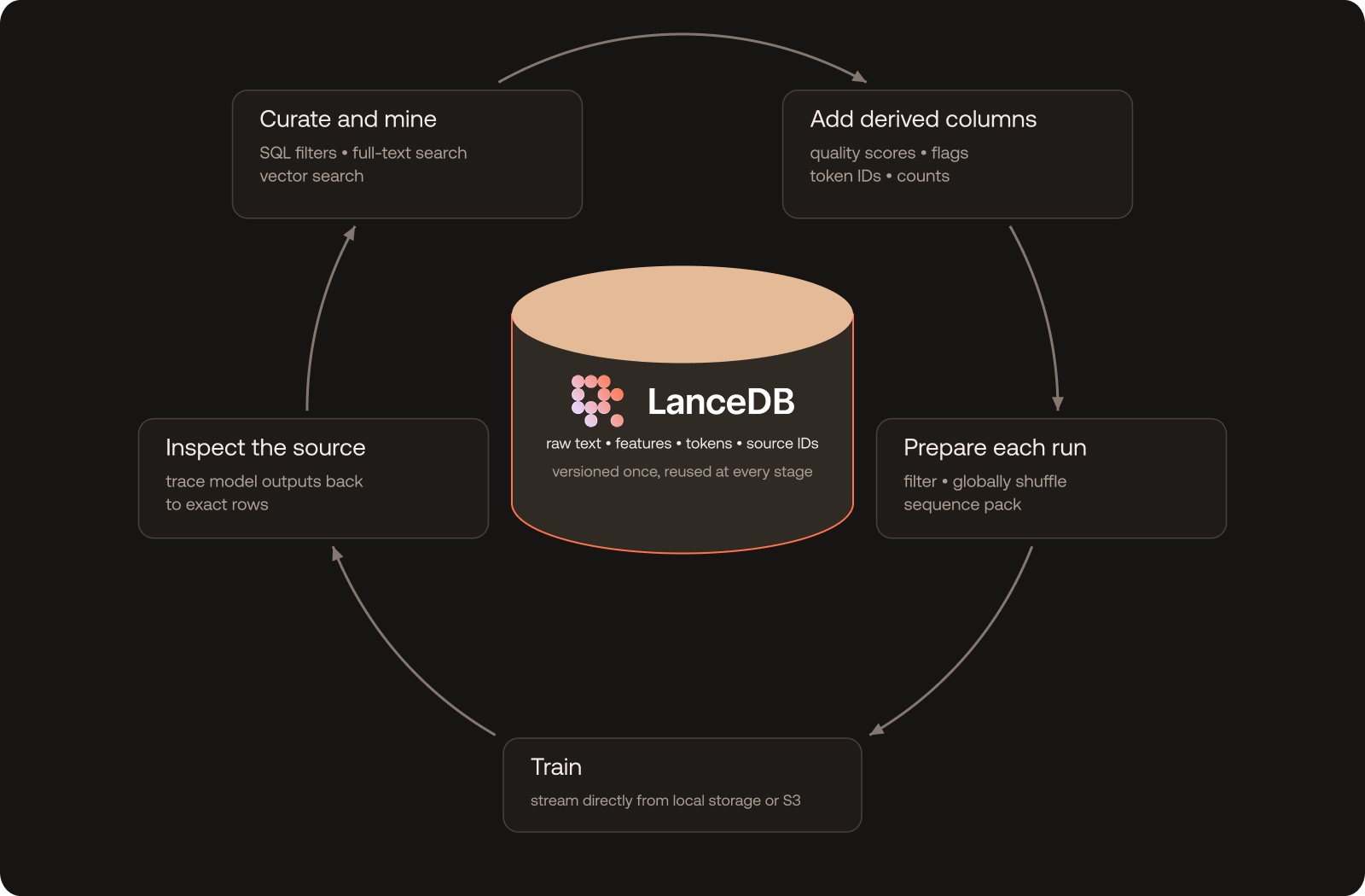
Because those steps operate on the same versioned rows, there are fewer copies to rebuild and fewer systems to keep in sync. The dataloader can filter, globally shuffle, and pack those rows directly from S3, while the table remains available for search and analysis.

On 8 H100s, this pipeline goes from raw text to a trained 124M model in 25 minutes. It matches pre-packed loaders at 3.18M tokens per second, can resume on a different number of GPUs, and scales to a 354M model trained on 7B tokens in 97 minutes. Reproduction code and additional training examples are available in the training repository.