
Start with 10 million vectors. Grow to billions. Keep the freedom to choose how you search.
A search feature rarely stands still. An image browser becomes a recommendation system. A retrieval pipeline needs better matches. New embeddings keep arriving, and the table grows from millions of vectors to billions.
LanceDB is built for that journey, with compact, efficient search at 10 million vectors, distributed indexing as the table grows, and responsive queries at 10-billion vector scale. The same table can also support offline analysis, with storage and query-time precision controls that adapt to each workload.
Start with 10 million vectors
We started with 10 million 768-dimensional image embeddings, comparing RaBitQ (RQ), product quantization (PQ), and scalar quantization (SQ). We tested two PQ configurations, PQ96 and PQ384, alongside one-bit and five-bit RQ and SQ, all without raw-vector refinement.
Using five-bit RaBitQ, LanceDB's underlying Lance engine reached 1,614 QPS at 96.2% recall. PQ96 reached 1,647 QPS at 68.6% recall, while PQ384 reached 1,047 QPS at 91.5% recall. Five-bit RQ combined higher recall than either PQ configuration with throughput close to PQ96 and 1.54× that of PQ384.
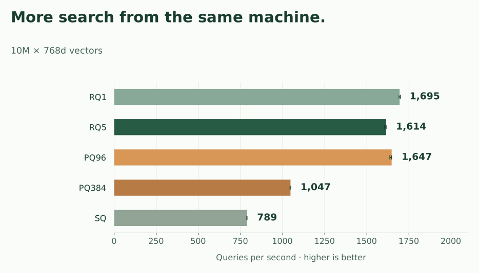
For teams running search all day, that efficiency translates into more requests from the same infrastructure budget. LanceDB's five-bit RaBitQ search reaches this quality directly from compressed vectors, without an extra pass over the original vectors.
RaBitQ combines compact codes with selective scoring. LanceDB starts with a cheap one-bit distance bound to eliminate unpromising candidates, then uses additional bits only for the survivors. In one profiled workload, this pruning step eliminated about 99.9% of candidate rows once the result threshold tightened. That helps five-bit RQ deliver higher recall without multiplying query time by the number of bits.
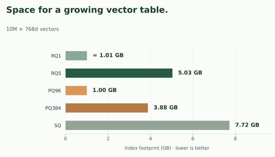
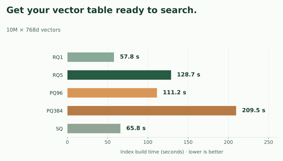
Storage and build speed add two more dimensions to the choice. The estimated one-bit RQ footprint is one fifth that of five-bit RQ, while five-bit RQ retains more detail for higher recall.
From millions to billions
Ten million vectors is a starting point. As new images, documents, and embeddings arrive, the same table can grow to hundreds of millions, 10 billion vectors, and beyond. Efficient queries are only part of the challenge because the index also has to keep up as the table grows.
Keep indexing as the table grows
A first index build is only the beginning. LanceDB scales both the initial build and the work of keeping an index current.
Start with a parallel build. LanceDB distributes the initial indexing work across machines. Workers build different segments of your table at the same time, and LanceDB publishes the completed index together.
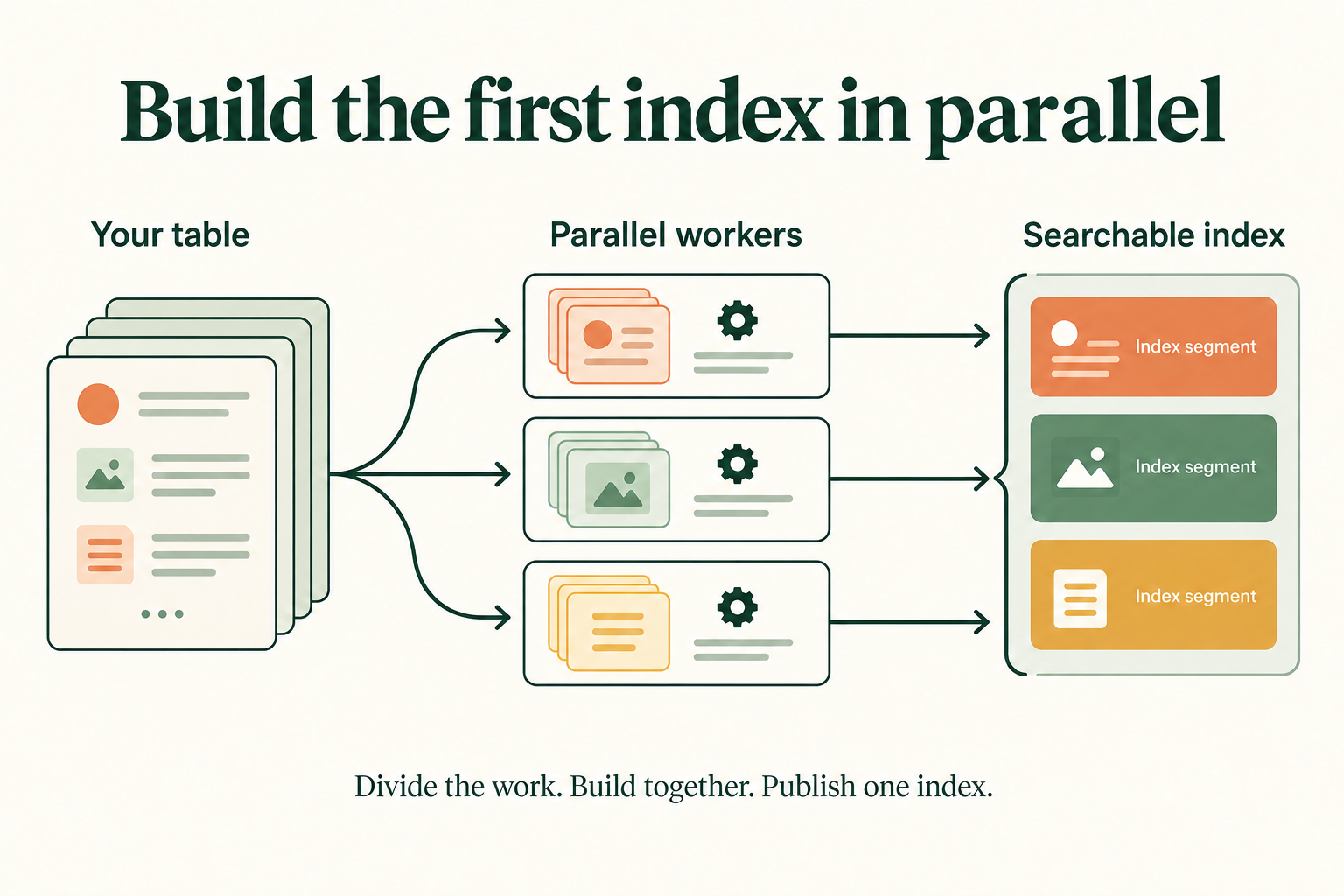
Then keep up with new data. Once your historical data is indexed, LanceDB adapts index maintenance to the size of each addition.
- Small additions: LanceDB uses SPFresh to merge new data into the tail and rebalance its IVF partitions, helping maintain low tail latency and high recall as data arrives.
- Larger additions: LanceDB builds multiple new segments in parallel across distributed workers, speeding up indexing for large batches.
- A growing tail: LanceDB can replace it with two segments while keeping the rest of the index in place.
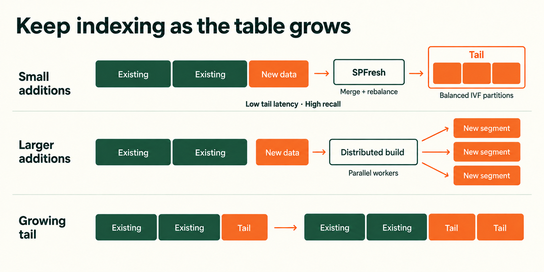
For example, you can add a fresh batch of images to an existing table without routinely rebuilding all of its historical segments. LanceDB chooses the maintenance path based on the new batch and the existing index, and publishes completed changes together.
That gives teams a practical path from the first large import to the next day's updates and the next billion vectors.
10 billion vectors. Over 1,000 queries per second.
A growing table should leave room for a growing audience. LanceDB’s distributed search architecture puts multiple machines to work behind a single search experience.
For this test, we created the 10-billion-vector dataset by repeating the 10-million-vector dataset 1,000 times. Across these 10 billion 768-dimensional index entries, median response time was 18.05 ms, with 21.61 ms at p99.
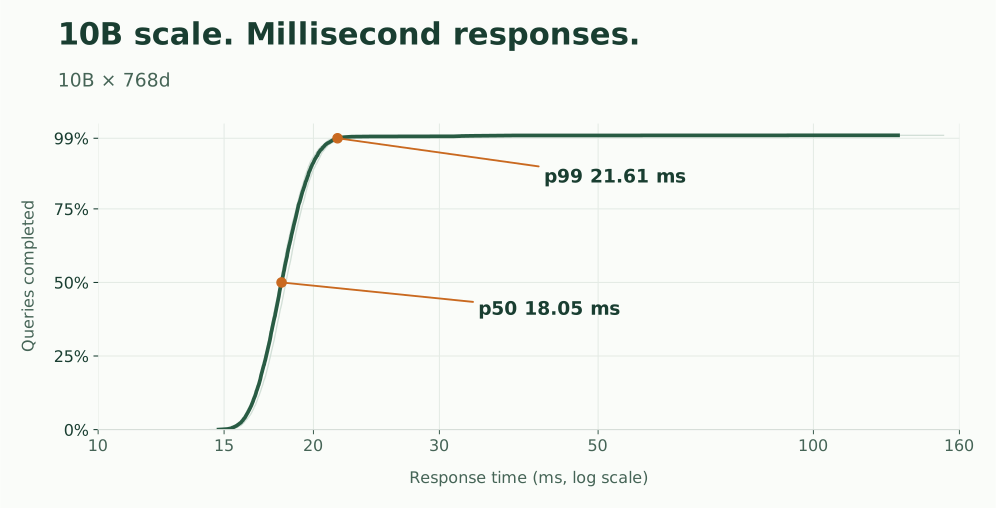
With nprobes=20, throughput reached 951 queries per second at 32 concurrent requests. Increasing concurrency to 256 raised throughput to 1,066 queries per second. Search runs across segments in parallel, and their candidates come together as one result.
This allows for the capacity to serve more searches as vector tables grow.
One table. Online and offline search.
An interactive search and an offline retrieval job can ask different things of the same table. LanceDB lets each request choose its balance of speed and precision through query-time controls, without rebuilding the index.
Choose precision when you query. On a five-bit RaBitQ index, fast scores candidates using one bit per dimension. That is one fifth of the stored code bits. The normal mode can use all five bits to calculate more accurate distances and improve recall.
More precision does not mean scoring every candidate with all five bits. RaBitQ first evaluates a one-bit distance lower bound to prune candidates that cannot improve the current results. Only the survivors need the additional four bits. Once the result threshold tightens, pruning can eliminate over 99% of candidates—so even normal can reject the vast majority using only the one-bit layer.
On the 10M × 768d workload, switching from fast to normal raised recall from 75.0% to 93.1% at the same search breadth, while both modes sustained approximately 1,700 QPS. This selective use of the extra bits motivates keeping the one-bit layer close to the CPU and placing the additional precision on a larger storage tier.
Match the storage tier to the workload. LanceDB Enterprise combines memory, local NVMe SSD, and object storage. Memory serves hot index data for responsive online queries. Local NVMe extends the working set for deeper searches and offline jobs. Object storage durably holds the complete table and indexes.
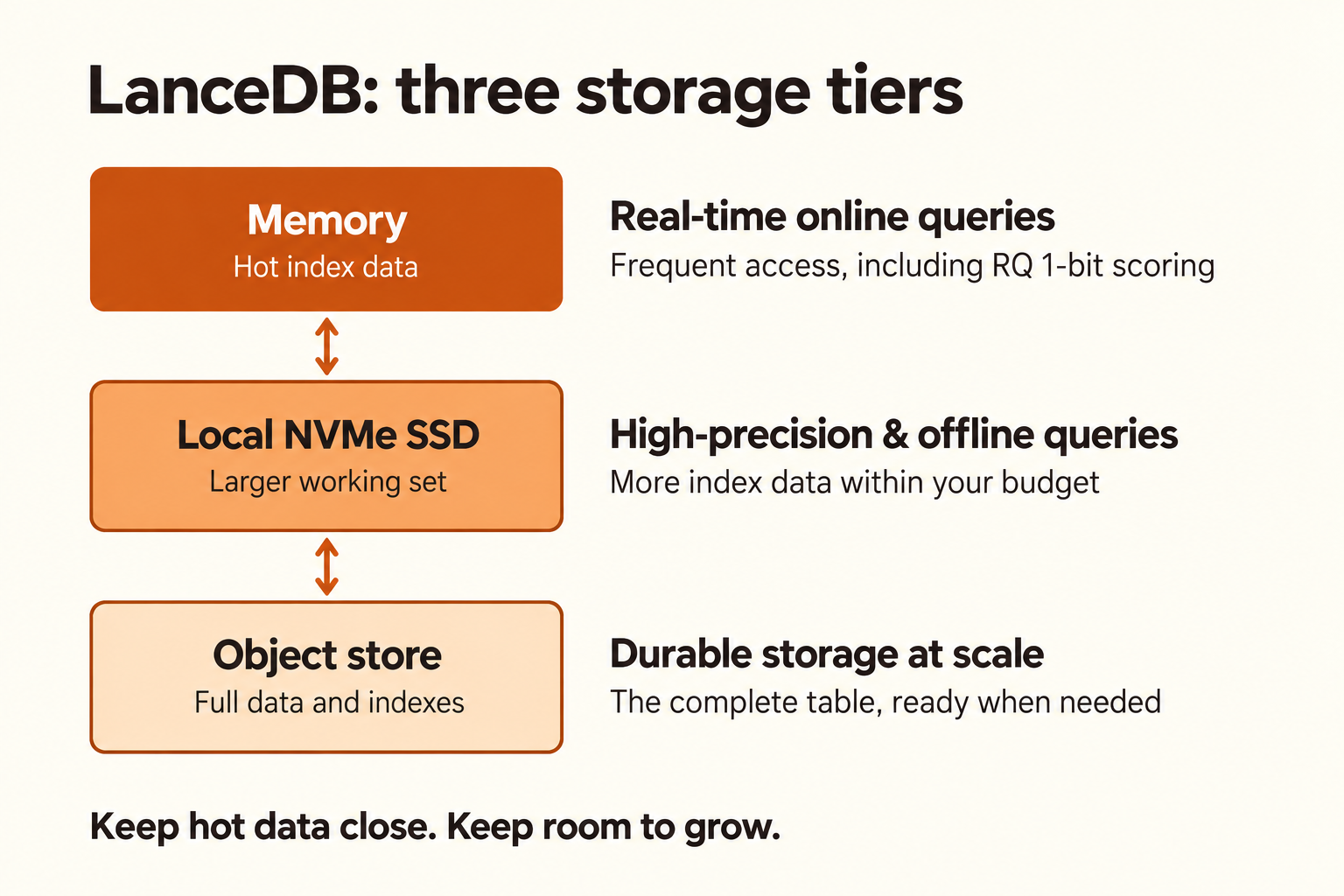
To see the capacity trade-off, consider two illustrative placements of the code payload for 10B × 768d vectors:
With candidate-selective fetching, the split layout would perform pruning in RAM and read the extra bits from NVMe only for survivors. It would not require a disk read for every candidate, and its code payload would need one fifth as much RAM.
Query-time precision and configurable memory/NVMe cache budgets give teams two ways to adapt search to the request, letting them spend scoring work on the quality needed while sizing the working set for the online or offline workload.
Build for your next workload.
Different search and retrieval workloads do not all need the same balance of speed and precision. LanceDB lets each request choose the supported scoring mode and search breadth that fit its needs, while configurable cache budgets help the deployment fit the workload.
For applications that prioritize retrieval quality, build a RaBitQ index with up to 9 bits per dimension. The additional bits preserve more detail in the compressed representation for high-precision search. Query-time controls then let you choose between faster scoring and the higher-fidelity paths supported by that index.
That flexibility carries forward as your application grows, supporting responsive online queries, deeper offline searches, and distributed and incremental indexing that keeps new data searchable.
Start with the table you have today. LanceDB gives you room to grow.